Code
%load_ext autoreload
%autoreload 2Picking out combinations of action (forecast, limited to 3 days) and observational triggers. All trigger combination options have the same overall return period (3.7 years, which is 7 triggering years in the period 2000-2024).
We varied, each for the forecast and the observational:
mean, or quantiles 50, 80, 90, 95)And we are looking to optimize for (maximizing):
Total Affected from EM-DAT for the triggered stormsAmount in US$ from CERF for the triggered storms%load_ext autoreload
%autoreload 2import ocha_stratus as stratus
import pandas as pd
import matplotlib.pyplot as plt
import matplotlib.patches as mpatches
from src.datasources import ibtracs
from src.datasources.ibtracs import knots2cat
from src.constants import *Load the trigger metrics dataset that was generated from the optimization process. This contains all valid trigger combinations that meet the 3.7-year return period requirement, along with their associated impact metrics.
blob_name = (
    f"{PROJECT_PREFIX}/processed/fcast_obsv_combined_trigger_metrics.parquet"
)
df_metrics = stratus.load_parquet_from_blob(blob_name)Load the comprehensive dataset containing both forecast and observed storm statistics, along with impact data. This will be used to analyze individual storms and create detailed visualizations.
blob_name = f"{PROJECT_PREFIX}/processed/fcast_obsv_combined_stats.parquet"
df_stats = stratus.load_parquet_from_blob(blob_name)
Calculate the target number of years for CERF-related triggers, accounting for the fact that CERF funding only started in 2006. This adjusts the return period calculation to the available CERF timeframe.
### Calculate CERF Target Years
# note that we have to pick a differet number of triggered years for CERF since it only started in 2006
cerf_target_years = int((2024 - 2006 + 1 + 1) / 3.7)
Examine the years when CERF funding was provided and their associated funding amounts. This shows that there were 6 CERF years historically, but we can only target up to 5 to maintain the desired return period.
### Analyze Historical CERF Years
# we see that there were 6 CERF years, but we can only hope to target up to 5, because otherwise the RP is too low
df_stats[df_stats["cerf"]].groupby("year")[
    "Amount in US$"
].sum().reset_index().sort_values("Amount in US$", ascending=False)| year | Amount in US$ | |
|---|---|---|
| 5 | 2024 | 9499457 |
| 3 | 2017 | 7999469 |
| 4 | 2022 | 7827734 |
| 0 | 2008 | 7367516 |
| 1 | 2012 | 5522753 |
| 2 | 2016 | 5352736 |
Calculate the theoretical maximum CERF funding amount by selecting the top CERF years based on funding amount. This provides a benchmark for evaluating trigger performance.
### Calculate Maximum Possible CERF Amount

max_cerf_amount = (
    df_stats[df_stats["cerf"]]
    .groupby("year")["Amount in US$"]
    .sum()
    .reset_index()
    .sort_values("Amount in US$", ascending=False)
    .iloc[:cerf_target_years]
    .sum()["Amount in US$"]
)
Set the target number of years (7) for the main impact analysis, corresponding to the 3.7-year return period over the full analysis period from 2000-2024.
### Set Target Years for Impact Analysis
target_years = 7
Calculate the theoretical maximum total affected population by selecting the top 7 years (target years) with the highest affected populations. This benchmark helps evaluate how well different trigger combinations capture high-impact events.
### Calculate Maximum Possible Total Affected
max_total_affected = (
    df_stats.groupby("year")["Total Affected"]
    .sum()
    .reset_index()
    .sort_values("Total Affected", ascending=False)
    .iloc[:target_years]
    .sum()["Total Affected"]
)

max_total_affectednp.int64(29450226)Add new metrics to analyze the balance between forecast and observational triggers. These metrics help identify trigger combinations that favor one approach over the other or achieve balance between them.
df_metrics["n_years_diff"] = (
    df_metrics["n_years_fcast"] - df_metrics["n_years_obsv"]
)
df_metrics["n_years_diff_abs"] = df_metrics["n_years_diff"].abs()
df_metrics["n_years_total"] = (
    df_metrics["n_years_fcast"] + df_metrics["n_years_obsv"]
)
Create a utility function to remove redundant threshold combinations. For any given impact outcome, this function keeps only the lowest threshold values, eliminating trigger combinations that require unnecessarily high thresholds to achieve the same results.
### Define Function to Remove Redundant Thresholds
def drop_redundant_thresholds(df, min_cols, id_cols, drop_high=True):
    for min_col in min_cols:
        unique_cols = [x for x in min_cols if x != min_col] + id_cols
        df = df.sort_values(min_col, ascending=drop_high).drop_duplicates(
            subset=unique_cols
        )
    return df
Define the different types of columns for organizing the data: threshold columns (wind and rain thresholds), rainfall aggregation method columns, and impact metric columns.
### Define Column Categories

thresh_cols = [
    "fcast_wind",
    "fcast_rain_thresh",
    "obsv_wind",
    "obsv_rain_thresh",
]
rain_agg_cols = ["fcast_rain_col", "obsv_rain_col"]
impact_cols = [
    "Total Affected",
    "Total Deaths",
    "Total Damage, Adjusted ('000 US$)",
    "Amount in US$",
]
Apply the redundancy removal function to keep only the most efficient trigger combinations - those that achieve the same impact outcomes with the lowest possible thresholds.
df_metrics_lowest = drop_redundant_thresholds(
    df_metrics, thresh_cols, impact_cols + rain_agg_cols
)
Display the filtered dataset of non-redundant trigger combinations to see the reduced set of viable options.
### Display Filtered Results
df_metrics_lowest| Total Affected | Total Deaths | Total Damage, Adjusted ('000 US$) | Amount in US$ | cerf | fcast_wind | fcast_rain_col | fcast_rain_thresh | obsv_wind | obsv_rain_col | obsv_rain_thresh | n_years_fcast | n_years_obsv | n_years_diff | n_years_diff_abs | n_years_total | |
|---|---|---|---|---|---|---|---|---|---|---|---|---|---|---|---|---|
| 332720 | 24745221.0 | 41.0 | 8135595.0 | 23194719.0 | 4.0 | 80.0 | q50 | 41.205720 | 125.0 | q50_obsv | 2.44 | 7 | 4 | 3 | 3 | 11 |
| 198088 | 16341819.0 | 52.0 | 13714030.0 | 26242474.0 | 5.0 | 35.0 | q95 | 141.738710 | 125.0 | q50_obsv | 2.44 | 7 | 4 | 3 | 3 | 11 |
| 22746 | 24843276.0 | 41.0 | 11268506.0 | 28547455.0 | 5.0 | 120.0 | q80 | 70.166730 | 130.0 | q50_obsv | 2.44 | 7 | 4 | 3 | 3 | 11 |
| 82763 | 21735221.0 | 38.0 | 11280927.0 | 20719721.0 | 4.0 | 110.0 | q80 | 78.203220 | 115.0 | q50_obsv | 2.44 | 7 | 6 | 1 | 1 | 13 |
| 314406 | 21495776.0 | 38.0 | 8110595.0 | 15366985.0 | 3.0 | 75.0 | q50 | 42.807594 | 130.0 | q50_obsv | 2.44 | 7 | 4 | 3 | 3 | 11 |
| ... | ... | ... | ... | ... | ... | ... | ... | ... | ... | ... | ... | ... | ... | ... | ... | ... |
| 25202 | 24992721.0 | 45.0 | 12317493.0 | 28547455.0 | 5.0 | 120.0 | mean | 21.936502 | 30.0 | q80_obsv | NaN | 7 | 0 | 7 | 7 | 7 |
| 25203 | 24992721.0 | 45.0 | 12317493.0 | 28547455.0 | 5.0 | 120.0 | mean | 21.936502 | 30.0 | q95_obsv | NaN | 7 | 0 | 7 | 7 | 7 |
| 100940 | 16292374.0 | 52.0 | 13714030.0 | 26242474.0 | 5.0 | 90.0 | q95 | 140.547760 | 30.0 | mean_obsv | NaN | 7 | 0 | 7 | 7 | 7 |
| 100943 | 16292374.0 | 52.0 | 13714030.0 | 26242474.0 | 5.0 | 90.0 | q95 | 140.547760 | 30.0 | q80_obsv | NaN | 7 | 0 | 7 | 7 | 7 |
| 328878 | 24695776.0 | 41.0 | 8135595.0 | 23194719.0 | 4.0 | 80.0 | q50 | 41.205720 | 30.0 | q80_obsv | NaN | 7 | 0 | 7 | 7 | 7 |
2543 rows × 16 columns
Create a comprehensive plotting function for visualizing trigger combinations. This function creates scatter plots with various filtering options to explore different aspects of the trigger optimization results, including forecast preference, balanced approaches, and theoretical maximum lines.
def plot_thresh_scatter(
    x="Total Affected",
    y="Amount in US$",
    color="n_years_diff_abs",
    zorder_rev=True,
    fcast_pref_only=False,
    same_wind=False,
    same_rain_col=False,
    zero_intercept=False,
    df=None,  # override default dataframe
):
    fig, ax = plt.subplots(figsize=(7, 7))

    if df is None:
        df_plot = df_metrics_lowest.copy()
    else:
        df_plot = df.copy()

    if same_wind:
        df_plot = df_plot[df_plot["fcast_wind"] == df_plot["obsv_wind"]]
    if same_rain_col:
        df_plot = df_plot[
            df_plot["fcast_rain_col"]
            == df_plot["obsv_rain_col"].str.removesuffix("_obsv")
        ]

    if fcast_pref_only:
        df_plot = df_plot[df_plot["n_years_diff"] >= 0]

    for n_years_diff_abs, group in df_plot.groupby(color):
        group.plot(
            x=x,
            y=y,
            marker=".",
            linewidth=0,
            alpha=1,
            label=n_years_diff_abs,
            ax=ax,
            zorder=-n_years_diff_abs if zorder_rev else n_years_diff_abs,
        )

    ax.axhline(max_cerf_amount, linestyle="--", color="dodgerblue")
    ax.axvline(max_total_affected, linestyle="--", color="dodgerblue")

    if zero_intercept:
        ax.set_xlim(left=0)
        ax.set_ylim(bottom=0)

    ax.legend(title=color)
    ax.set_ylabel(y)
    ax.set_xlabel(x)
    ax.spines.top.set_visible(False)
    ax.spines.right.set_visible(False)

    return fig, ax
Calculate the maximum wind speed across both forecast and observed data to set appropriate plot limits.
### Get Maximum Wind Speed
max_wind = df_stats[["wind", "wind_obsv"]].max().max()
Create a utility function that applies a specific trigger combination to the storm dataset, adding flags to indicate which storms would be triggered by forecast conditions and which by observed conditions.
### Define Function to Get Triggered Storms
def get_triggered_storms(index):
    trig = df_metrics_lowest.loc[index]

    df_stats["fcast_trig"] = (df_stats["wind"] >= trig["fcast_wind"]) & (
        df_stats[trig["fcast_rain_col"]] >= trig["fcast_rain_thresh"]
    )

    df_stats["obsv_trig"] = (df_stats["wind_obsv"] >= trig["obsv_wind"]) & (
        df_stats[trig["obsv_rain_col"]] >= trig["obsv_rain_thresh"]
    )

    return df_stats
Create a comprehensive plotting function that visualizes individual trigger combinations. This function creates dual plots (forecast vs observed) showing storm positions relative to trigger thresholds, with bubble sizes representing impact levels and colors indicating CERF funding status.
def plot_selected_threshs(index, impact_col="Total Affected"):
    trig_color = "gold"
    cerf_color = "crimson"

    fig, axs = plt.subplots(1, 2, figsize=(14, 7), dpi=200)

    trig = df_metrics_lowest.loc[index]
    # print(trig)

    df_stats = get_triggered_storms(index)

    figs = []
    for stage, ax in zip(["fcast", "obsv"], axs):
        other_stage = "fcast" if stage == "obsv" else "obsv"
        wind_col = "wind" if stage == "fcast" else "wind_obsv"
        wind_thresh = trig[f"{stage}_wind"]
        rain_col = trig[f"{stage}_rain_col"]
        rain_thresh = trig[f"{stage}_rain_thresh"]

        ymax = df_stats[rain_col].max() * 1.1
        xmax = max_wind * 1.1

        # fig, ax = plt.subplots(dpi=200, figsize=(7, 7))

        bubble_sizes = df_stats[impact_col].fillna(0)
        bubble_sizes_scaled = bubble_sizes / bubble_sizes.max() * 5000

        ax.scatter(
            df_stats[wind_col],
            df_stats[rain_col],
            s=bubble_sizes_scaled,
            c=df_stats["cerf"].apply(lambda x: cerf_color if x else "grey"),
            alpha=0.3,
            edgecolor="none",
            zorder=1,
        )

        for _, row in df_stats.iterrows():
            triggered = row[f"{stage}_trig"]
            other_triggered = row[f"{other_stage}_trig"]
            ax.annotate(
                row["name"].capitalize() + "\n" + str(row["year"]),
                (row[wind_col], row[rain_col]),
                ha="center",
                va="center",
                fontsize=6,
                color=cerf_color if row["cerf"] == True else "k",
                zorder=10 if row["cerf"] else 9,
                alpha=0.8,
                fontstyle="italic" if other_triggered else "normal",
                fontweight="bold" if triggered else "normal",
            )

        ax.axvline(
            wind_thresh,
            color=trig_color,
            linewidth=0.5,
            zorder=0,
        )
        ax.axhline(
            rain_thresh,
            color=trig_color,
            linewidth=0.5,
            zorder=0,
        )
        ax.add_patch(
            mpatches.Rectangle(
                (wind_thresh, rain_thresh),  # bottom left
                xmax - wind_thresh,  # width
                ymax - rain_thresh,  # height
                facecolor=trig_color,
                alpha=0.1,
                zorder=0,
            )
        )

        for cat_value, cat_name in CAT_LIMITS:
            ax.annotate(
                cat_name + " -",
                (cat_value, 0),
                fontstyle="italic",
                color="grey",
                rotation=90,
                va="top",
                ha="center",
                fontsize=8,
            )

        ax.annotate(
            f" {wind_thresh:.0f} ",
            (wind_thresh, 0),
            color=trig_color,
            rotation=90,
            fontsize=10,
            va="top",
            ha="center",
            fontweight="bold",
        )

        ax.annotate(
            f" {rain_thresh:.1f} ",
            (0, rain_thresh),
            color=trig_color,
            fontsize=10,
            va="center",
            ha="right",
            fontweight="bold",
        )

        if rain_col == "mean":
            rain_agg_str = "mean"
        else:
            q = rain_col.removeprefix("q").removesuffix("_obsv")
            if q == "50":
                rain_agg_str = "median"
            else:
                rain_agg_str = f"{q}th quantile"
        ax.set_ylabel(
            f"Two-day rainfall, {rain_agg_str} over whole country (mm)"
        )
        ax.set_xlabel("\nMax. wind speed while in ZMA (knots)")

        ax.set_xlim(left=0, right=xmax)
        ax.set_ylim(bottom=0, top=ymax)

        ax.set_title(
            "Action (forecast)" if stage == "fcast" else "Observational"
        )

        ax.spines.top.set_visible(False)
        ax.spines.right.set_visible(False)

        # figs.append((fig, ax))
    return fig, axs
Create utility functions to format and display storm data in a clear, color-coded format. These functions help categorize CERF funding status and apply appropriate styling to data tables.
def set_cerf_str(row):
    if row["cerf"]:
        return "Yes"
    else:
        if row["year"] >= 2006:
            return "No"
        else:
            return "pre-"


def color_df(val):
    if val == "Yes":
        return "background-color: crimson"
    elif val == "No":
        return "background-color: dodgerblue"
    elif val == "Trig.":
        return "background-color: darkorange"
    else:
        return ""
Create a comprehensive table display function that shows which storms would be triggered by a specific trigger combination. The function creates a styled table with color coding for CERF status and trigger conditions, along with impact metrics.
### Define Detailed Storm Display Function

def disp_selected_threshs(index, impact_col="Total Affected"):
    trig_color = "gold"
    cerf_color = "crimson"

    df_disp = get_triggered_storms(index).copy()

    df_disp["CERF"] = df_disp.apply(set_cerf_str, axis=1)

    df_disp["Storm"] = (
        df_disp["name"].str.capitalize() + " " + df_disp["year"].astype(str)
    )
    df_disp["Action"] = df_disp["fcast_trig"].apply(
        lambda x: "Trig." if x else "No trig."
    )
    df_disp["Obsv."] = df_disp["obsv_trig"].apply(
        lambda x: "Trig." if x else "No trig."
    )

    cols = ["Action", "Obsv.", "CERF", impact_col]
    display(
        df_disp.set_index("Storm")[cols]
        .sort_values(impact_col, ascending=False)
        .style.bar(
            subset=impact_col,
            color="mediumpurple",
            # vmax=500000,
            props="width: 150px;",
        )
        .map(color_df)
        .set_table_styles(
            {
                impact_col: [
                    {"selector": "th", "props": [("text-align", "left")]},
                    {"selector": "td", "props": [("text-align", "left")]},
                ]
            }
        )
        .format({"Total Affected": "{:,}"})
)Generate a scatter plot showing the relationship between total affected population and CERF funding amounts for different trigger combinations. The horizontal line at 2.8e7 helps identify high-CERF threshold combinations.
The cluster (option 1 in slides) where the same number of years are triggered with forecast and observational.
fig, ax = plot_thresh_scatter(
    "Total Affected", "Amount in US$", "n_years_diff_abs"
)
ax.axhline(2.8e7)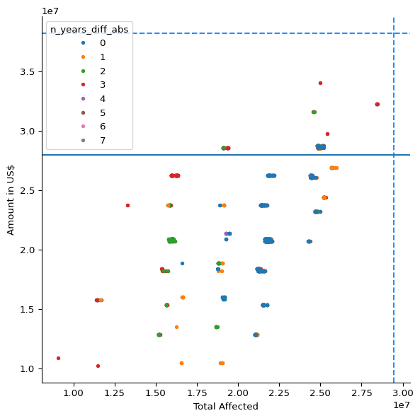
Extract trigger combinations where the forecast and observational approaches trigger the same number of years (difference of 0), representing balanced trigger strategies.
df_metrics_balanced = df_metrics_lowest[
    df_metrics_lowest["n_years_diff_abs"] == 0
]From the balanced combinations, select those with high CERF funding amounts (>=2.8e7) to identify the best balanced trigger options.
df_metrics_balanced_high = df_metrics_balanced[
    df_metrics_balanced["Amount in US$"] >= 2.8e7
]
Show the filtered set of balanced trigger combinations with high CERF funding potential.
df_metrics_balanced_high| Total Affected | Total Deaths | Total Damage, Adjusted ('000 US$) | Amount in US$ | cerf | fcast_wind | fcast_rain_col | fcast_rain_thresh | obsv_wind | obsv_rain_col | obsv_rain_thresh | n_years_fcast | n_years_obsv | n_years_diff | n_years_diff_abs | n_years_total | |
|---|---|---|---|---|---|---|---|---|---|---|---|---|---|---|---|---|
| 71389 | 24843276.0 | 41.0 | 11268506.0 | 28547455.0 | 5.0 | 110.0 | q95 | 143.712340 | 105.0 | q50_obsv | 45.957497 | 5 | 5 | 0 | 0 | 10 |
| 119458 | 25087281.0 | 45.0 | 12817901.0 | 28547455.0 | 5.0 | 100.0 | q95 | 143.712340 | 105.0 | q50_obsv | 45.957497 | 5 | 5 | 0 | 0 | 10 |
| 119486 | 25187281.0 | 49.0 | 13866888.0 | 28547455.0 | 5.0 | 100.0 | q95 | 143.409800 | 105.0 | q50_obsv | 45.957497 | 5 | 5 | 0 | 0 | 10 |
| 71417 | 24943276.0 | 45.0 | 12317493.0 | 28547455.0 | 5.0 | 110.0 | q95 | 143.409800 | 105.0 | q50_obsv | 45.957497 | 5 | 5 | 0 | 0 | 10 |
| 60832 | 24865326.0 | 52.0 | 8098174.0 | 28717472.0 | 5.0 | 120.0 | q50 | 26.483074 | 75.0 | q50_obsv | 45.957497 | 6 | 6 | 0 | 0 | 12 |
| 60935 | 24815881.0 | 52.0 | 8098174.0 | 28717472.0 | 5.0 | 120.0 | q50 | 28.462177 | 75.0 | q50_obsv | 45.957497 | 6 | 6 | 0 | 0 | 12 |
| 191429 | 25154827.0 | 57.0 | 9647569.0 | 28717472.0 | 5.0 | 35.0 | q80 | 96.462585 | 105.0 | q80_obsv | 96.369003 | 5 | 5 | 0 | 0 | 10 |
| 98070 | 25109331.0 | 56.0 | 9647569.0 | 28717472.0 | 5.0 | 90.0 | q80 | 87.754250 | 105.0 | q80_obsv | 96.369003 | 5 | 5 | 0 | 0 | 10 |
| 313372 | 24865326.0 | 52.0 | 8098174.0 | 28717472.0 | 5.0 | 75.0 | q80 | 103.080360 | 105.0 | q80_obsv | 96.369003 | 5 | 5 | 0 | 0 | 10 |
| 191479 | 24910822.0 | 53.0 | 8098174.0 | 28717472.0 | 5.0 | 35.0 | q80 | 103.080360 | 105.0 | q80_obsv | 96.369003 | 5 | 5 | 0 | 0 | 10 |
| 312969 | 24865326.0 | 52.0 | 8098174.0 | 28717472.0 | 5.0 | 75.0 | mean | 59.768433 | 105.0 | q80_obsv | 96.369003 | 5 | 5 | 0 | 0 | 10 |
| 313322 | 25109331.0 | 56.0 | 9647569.0 | 28717472.0 | 5.0 | 75.0 | q80 | 96.462585 | 105.0 | q80_obsv | 96.369003 | 5 | 5 | 0 | 0 | 10 |
| 191184 | 24910822.0 | 53.0 | 8098174.0 | 28717472.0 | 5.0 | 35.0 | mean | 59.768433 | 105.0 | q80_obsv | 96.369003 | 5 | 5 | 0 | 0 | 10 |
Create detailed plots showing how the selected balanced trigger combination (index 60832) would perform, displaying both forecast and observational trigger conditions.
plot_selected_threshs(60832)(<Figure size 2800x1400 with 2 Axes>,
array([<Axes: title={'center': 'Action (forecast)'}, xlabel='\nMax. wind speed while in ZMA (knots)', ylabel='Two-day rainfall, median over whole country (mm)'>,
<Axes: title={'center': 'Observational'}, xlabel='\nMax. wind speed while in ZMA (knots)', ylabel='Two-day rainfall, median over whole country (mm)'>],
dtype=object))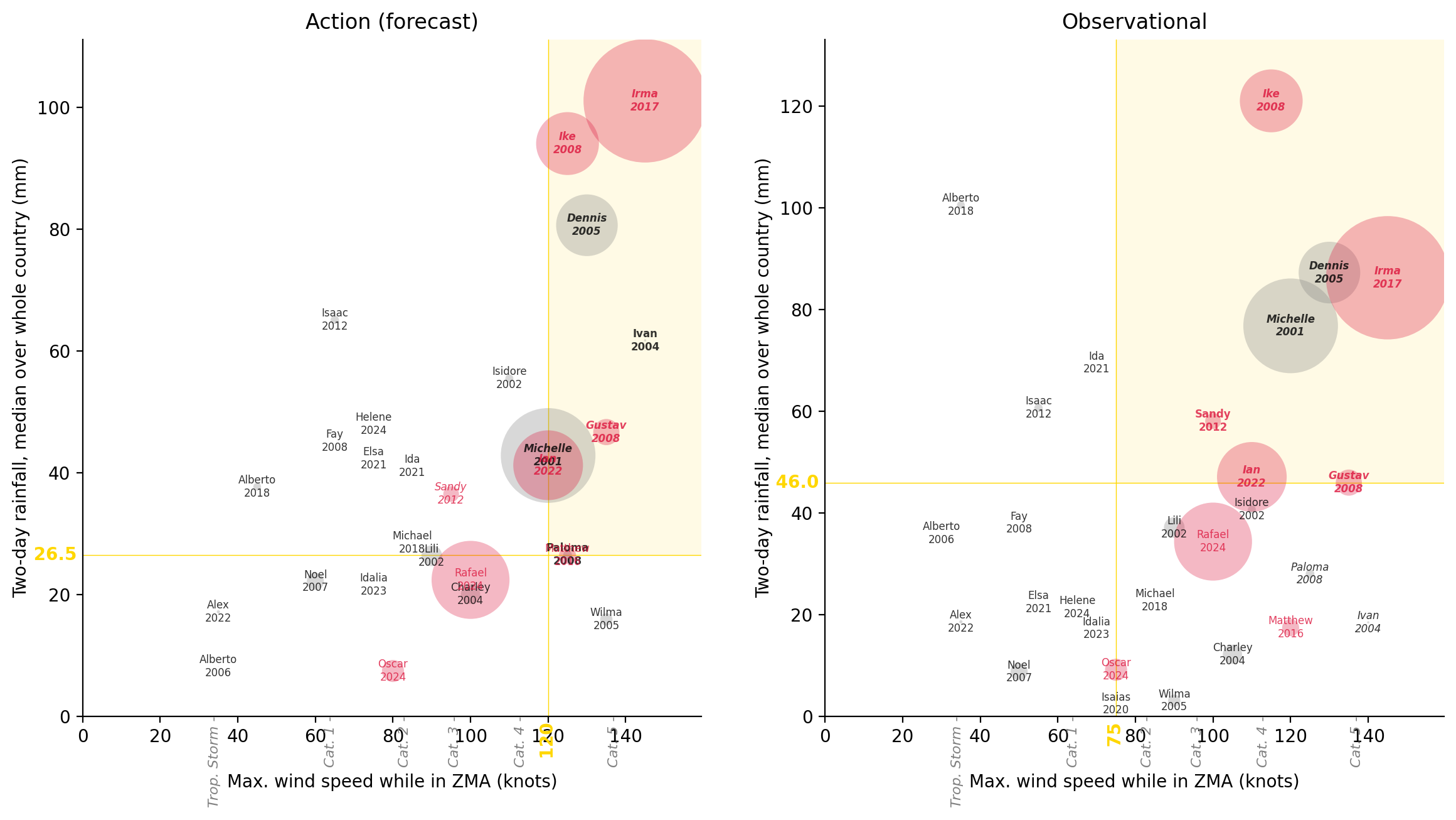
Show which specific storms would be triggered by this balanced combination, with detailed impact metrics and CERF funding information.
Cluster (option 2 in slides) maximizing impact
Generate a scatter plot with a vertical line at 2.7e7 to identify trigger combinations that maximize total affected population.
fig, ax = plot_thresh_scatter(
    "Total Affected", "Amount in US$", "n_years_diff_abs"
)
ax.axvline(2.7e7)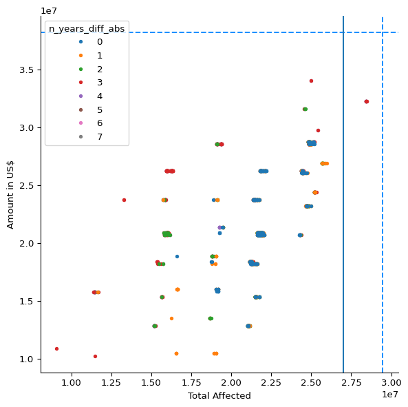
Select trigger combinations that achieve high total affected population (>=2.7e7) to identify options that maximize humanitarian impact.
### Filter for High-Impact Trigger Combinations
df_metrics_high_impact = df_metrics_lowest[
    df_metrics_lowest["Total Affected"] >= 2.7e7
]
Show the filtered set of trigger combinations that maximize total affected population.
### Display High-Impact Combinations
df_metrics_high_impact| Total Affected | Total Deaths | Total Damage, Adjusted ('000 US$) | Amount in US$ | cerf | fcast_wind | fcast_rain_col | fcast_rain_thresh | obsv_wind | obsv_rain_col | obsv_rain_thresh | n_years_fcast | n_years_obsv | n_years_diff | n_years_diff_abs | n_years_total | |
|---|---|---|---|---|---|---|---|---|---|---|---|---|---|---|---|---|
| 201131 | 28412062.0 | 52.0 | 4971882.0 | 32229929.0 | 5.0 | 35.0 | mean | 71.266540 | 75.0 | q80_obsv | 96.369003 | 4 | 7 | -3 | 3 | 11 |
| 201388 | 28412062.0 | 52.0 | 4971882.0 | 32229929.0 | 5.0 | 35.0 | q80 | 128.088730 | 75.0 | q80_obsv | 96.369003 | 3 | 7 | -4 | 4 | 10 |
| 213486 | 28412062.0 | 52.0 | 4971882.0 | 32229929.0 | 5.0 | NaN | q80 | 35.698547 | 75.0 | q80_obsv | 96.369003 | 0 | 7 | -7 | 7 | 7 |
| 201218 | 28412062.0 | 52.0 | 4971882.0 | 32229929.0 | 5.0 | 35.0 | q50 | 80.616330 | 75.0 | q80_obsv | 96.369003 | 3 | 7 | -4 | 4 | 10 |
| 321926 | 28412062.0 | 52.0 | 4971882.0 | 32229929.0 | 5.0 | 75.0 | q50 | 65.069570 | 75.0 | q80_obsv | 96.369003 | 3 | 7 | -4 | 4 | 10 |
| 321743 | 28412062.0 | 52.0 | 4971882.0 | 32229929.0 | 5.0 | 75.0 | mean | 69.391884 | 75.0 | q80_obsv | 96.369003 | 4 | 7 | -3 | 3 | 11 |
| 201286 | 28457558.0 | 53.0 | 4971882.0 | 32229929.0 | 5.0 | 35.0 | q50 | 65.069570 | 75.0 | q80_obsv | 96.369003 | 4 | 7 | -3 | 3 | 11 |
| 213390 | 28412062.0 | 52.0 | 4971882.0 | 32229929.0 | 5.0 | NaN | q50 | 7.418959 | 75.0 | q80_obsv | 96.369003 | 0 | 7 | -7 | 7 | 7 |
| 214074 | 28412062.0 | 52.0 | 4971882.0 | 32229929.0 | 5.0 | NaN | q95 | 67.368840 | 75.0 | q80_obsv | 96.369003 | 0 | 7 | -7 | 7 | 7 |
| 213054 | 28412062.0 | 52.0 | 4971882.0 | 32229929.0 | 5.0 | NaN | mean | 21.936502 | 75.0 | q80_obsv | 96.369003 | 0 | 7 | -7 | 7 | 7 |
| 201114 | 28457558.0 | 53.0 | 4971882.0 | 32229929.0 | 5.0 | 35.0 | mean | 69.391884 | 75.0 | q80_obsv | 96.369003 | 4 | 7 | -3 | 3 | 11 |
| 170489 | 28412062.0 | 52.0 | 4971882.0 | 32229929.0 | 5.0 | 130.0 | q95 | 177.149400 | 75.0 | q80_obsv | 96.369003 | 1 | 7 | -6 | 6 | 8 |
| 201608 | 28412062.0 | 52.0 | 4971882.0 | 32229929.0 | 5.0 | 35.0 | q95 | 263.916200 | 75.0 | q80_obsv | 96.369003 | 1 | 7 | -6 | 6 | 8 |
Create detailed plots for the selected high-impact trigger combination (index 321743) showing both forecast and observational trigger conditions.
plot_selected_threshs(321743)(<Figure size 2800x1400 with 2 Axes>,
array([<Axes: title={'center': 'Action (forecast)'}, xlabel='\nMax. wind speed while in ZMA (knots)', ylabel='Two-day rainfall, mean over whole country (mm)'>,
<Axes: title={'center': 'Observational'}, xlabel='\nMax. wind speed while in ZMA (knots)', ylabel='Two-day rainfall, 80th quantile over whole country (mm)'>],
dtype=object))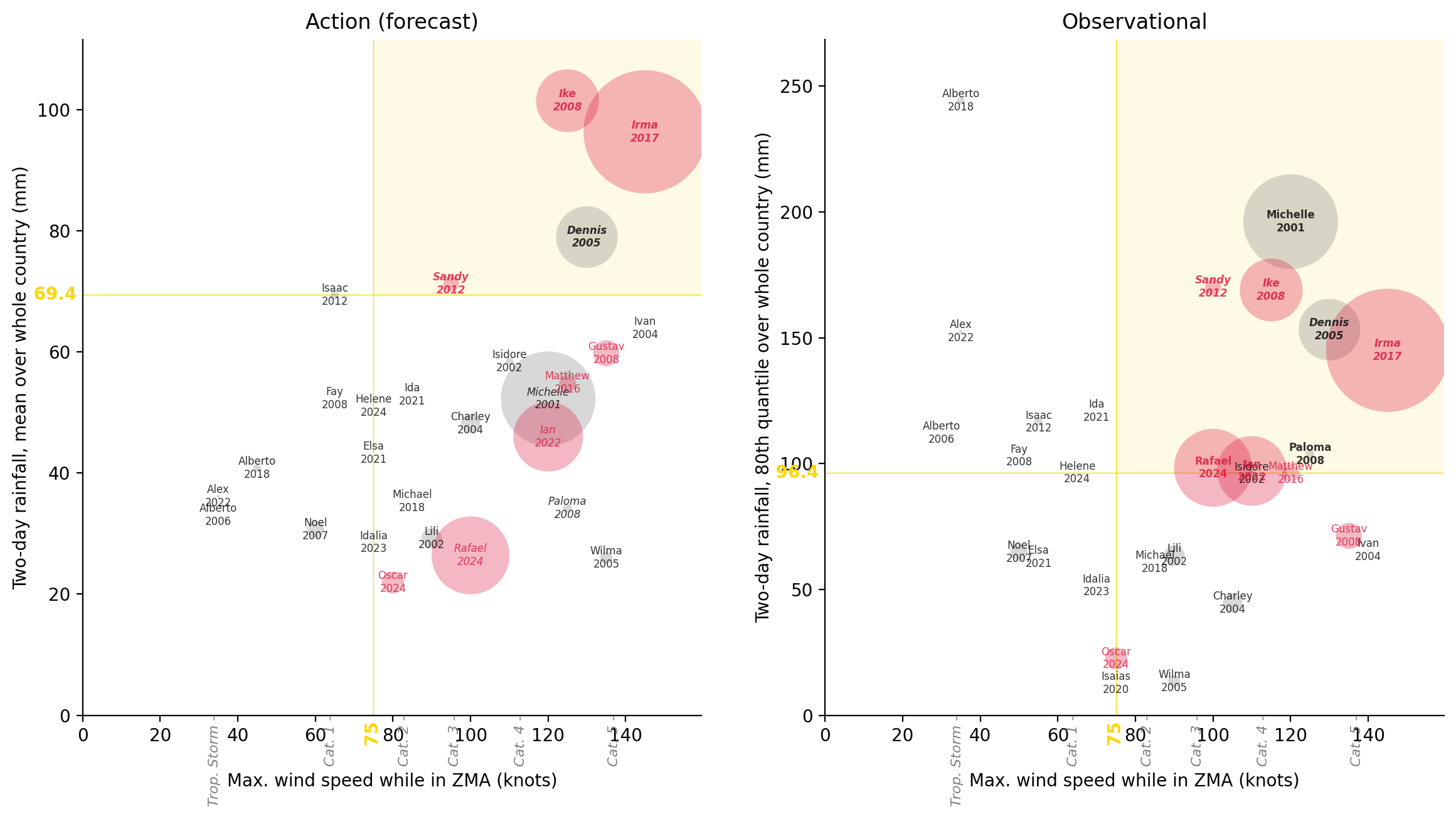
Show which specific storms would be triggered by this high-impact combination, with detailed impact metrics.
### Display Storm Details for High-Impact Combination
disp_selected_threshs(321743)| Action | Obsv. | CERF | Total Affected | |
|---|---|---|---|---|
| Storm | ||||
| Irma 2017 | Trig. | Trig. | Yes | 10,000,000 |
| Michelle 2001 | No trig. | Trig. | pre- | 5,900,012 |
| Rafael 2024 | No trig. | Trig. | Yes | 4,000,000 |
| Ian 2022 | No trig. | Trig. | Yes | 3,200,000 |
| Ike 2008 | Trig. | Trig. | Yes | 2,600,000 |
| Dennis 2005 | Trig. | Trig. | pre- | 2,500,000 |
| Gustav 2008 | No trig. | No trig. | Yes | 450,019 |
| Oscar 2024 | No trig. | No trig. | Yes | 320,000 |
| Lili 2002 | No trig. | No trig. | pre- | 281,470 |
| Charley 2004 | No trig. | No trig. | pre- | 244,005 |
| Noel 2007 | No trig. | No trig. | No | 192,488 |
| Matthew 2016 | No trig. | No trig. | Yes | 190,000 |
| Sandy 2012 | Trig. | Trig. | Yes | 162,605 |
| Wilma 2005 | No trig. | No trig. | pre- | 100,000 |
| Paloma 2008 | No trig. | Trig. | No | 49,445 |
| Isaac 2012 | No trig. | No trig. | No | 45,496 |
| Isidore 2002 | No trig. | No trig. | pre- | 42,500 |
| Alberto 2018 | No trig. | No trig. | No | 40,000 |
| Alex 2022 | No trig. | No trig. | No | 6,780 |
| Ivan 2004 | No trig. | No trig. | pre- | 3,245 |
| Michael 2018 | No trig. | No trig. | No | 540 |
| Isaias 2020 | No trig. | No trig. | No | 500 |
| Alberto 2006 | No trig. | No trig. | No | 268 |
| Ida 2021 | No trig. | No trig. | No | 0 |
| Elsa 2021 | No trig. | No trig. | No | 0 |
| Idalia 2023 | No trig. | No trig. | No | 0 |
| Helene 2024 | No trig. | No trig. | No | 0 |
| Dean 2007 | No trig. | No trig. | No | 0 |
| Fay 2008 | No trig. | No trig. | No | 0 |
Cluster (option 3 in slides) maximizing CERF amount
Generate a scatter plot with a horizontal line at 3.3e7 to identify trigger combinations that maximize CERF funding capture.
fig, ax = plot_thresh_scatter(
    "Total Affected", "Amount in US$", "n_years_diff_abs"
)
ax.axhline(3.3e7)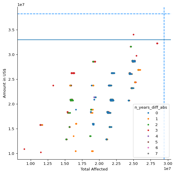
Select trigger combinations that achieve high CERF funding amounts (>=3.3e7) to identify options that maximize funding capture.
### Filter for High-CERF Trigger Combinations
df_metrics_high_cerf = df_metrics_lowest[
    df_metrics_lowest["Amount in US$"] >= 3.3e7
]
Show the filtered set of trigger combinations that maximize CERF funding capture.
### Display High-CERF Combinations
df_metrics_high_cerf| Total Affected | Total Deaths | Total Damage, Adjusted ('000 US$) | Amount in US$ | cerf | fcast_wind | fcast_rain_col | fcast_rain_thresh | obsv_wind | obsv_rain_col | obsv_rain_thresh | n_years_fcast | n_years_obsv | n_years_diff | n_years_diff_abs | n_years_total | |
|---|---|---|---|---|---|---|---|---|---|---|---|---|---|---|---|---|
| 201619 | 25002636.0 | 52.0 | 10958627.0 | 34070208.0 | 6.0 | 35.0 | q95 | 241.6073 | 75.0 | q50_obsv | 45.957497 | 2 | 6 | -4 | 4 | 8 |
| 91667 | 25002636.0 | 52.0 | 10958627.0 | 34070208.0 | 6.0 | 110.0 | q95 | 177.1494 | 75.0 | q50_obsv | 45.957497 | 3 | 6 | -3 | 3 | 9 |
Create detailed plots for the selected high-CERF trigger combination (index 91667) showing both forecast and observational trigger conditions.
plot_selected_threshs(91667)(<Figure size 2800x1400 with 2 Axes>,
array([<Axes: title={'center': 'Action (forecast)'}, xlabel='\nMax. wind speed while in ZMA (knots)', ylabel='Two-day rainfall, 95th quantile over whole country (mm)'>,
<Axes: title={'center': 'Observational'}, xlabel='\nMax. wind speed while in ZMA (knots)', ylabel='Two-day rainfall, median over whole country (mm)'>],
dtype=object))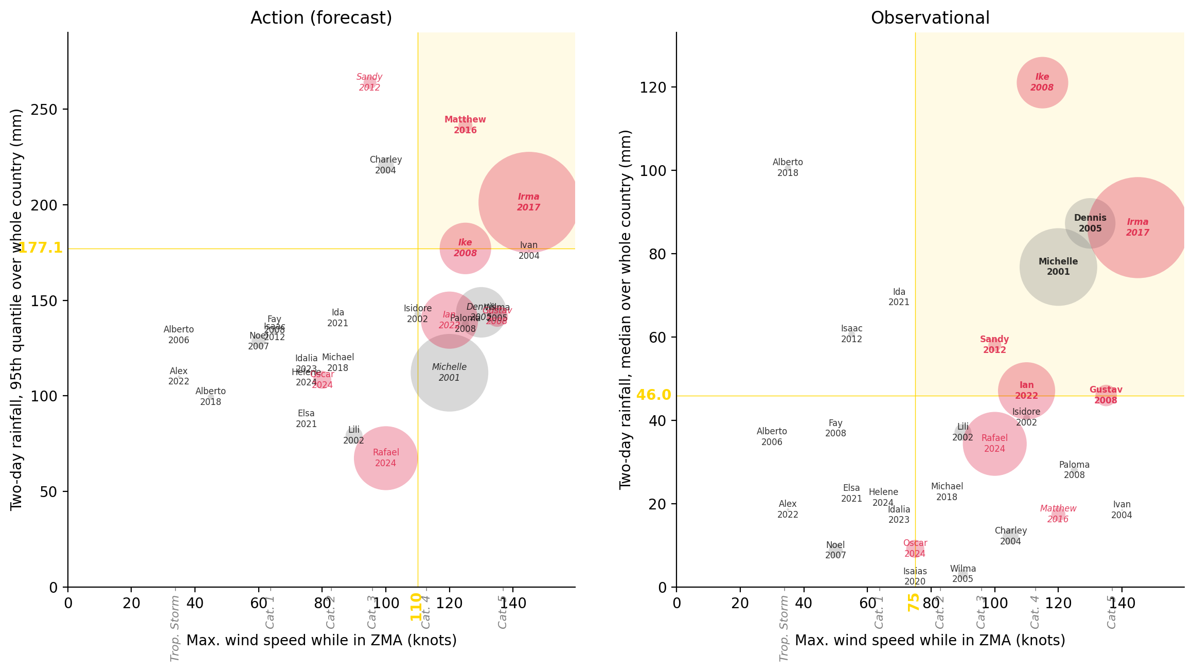
Show which specific storms would be triggered by this high-CERF combination, with detailed impact metrics and funding information.
### Display Storm Details for High-CERF Combination
disp_selected_threshs(91667)| Action | Obsv. | CERF | Total Affected | |
|---|---|---|---|---|
| Storm | ||||
| Irma 2017 | Trig. | Trig. | Yes | 10,000,000 |
| Michelle 2001 | No trig. | Trig. | pre- | 5,900,012 |
| Rafael 2024 | No trig. | No trig. | Yes | 4,000,000 |
| Ian 2022 | No trig. | Trig. | Yes | 3,200,000 |
| Ike 2008 | Trig. | Trig. | Yes | 2,600,000 |
| Dennis 2005 | No trig. | Trig. | pre- | 2,500,000 |
| Gustav 2008 | No trig. | Trig. | Yes | 450,019 |
| Oscar 2024 | No trig. | No trig. | Yes | 320,000 |
| Lili 2002 | No trig. | No trig. | pre- | 281,470 |
| Charley 2004 | No trig. | No trig. | pre- | 244,005 |
| Noel 2007 | No trig. | No trig. | No | 192,488 |
| Matthew 2016 | Trig. | No trig. | Yes | 190,000 |
| Sandy 2012 | No trig. | Trig. | Yes | 162,605 |
| Wilma 2005 | No trig. | No trig. | pre- | 100,000 |
| Paloma 2008 | No trig. | No trig. | No | 49,445 |
| Isaac 2012 | No trig. | No trig. | No | 45,496 |
| Isidore 2002 | No trig. | No trig. | pre- | 42,500 |
| Alberto 2018 | No trig. | No trig. | No | 40,000 |
| Alex 2022 | No trig. | No trig. | No | 6,780 |
| Ivan 2004 | No trig. | No trig. | pre- | 3,245 |
| Michael 2018 | No trig. | No trig. | No | 540 |
| Isaias 2020 | No trig. | No trig. | No | 500 |
| Alberto 2006 | No trig. | No trig. | No | 268 |
| Ida 2021 | No trig. | No trig. | No | 0 |
| Elsa 2021 | No trig. | No trig. | No | 0 |
| Idalia 2023 | No trig. | No trig. | No | 0 |
| Helene 2024 | No trig. | No trig. | No | 0 |
| Dean 2007 | No trig. | No trig. | No | 0 |
| Fay 2008 | No trig. | No trig. | No | 0 |
Looking at that little cluster with a two-year difference. Doesn’t look that remarkable, so left out of slides
Explore trigger combinations with a two-year difference between forecast and observational triggers, focusing on those with high CERF funding potential.
### Analyze Two-Year Difference Combinations
fig, ax = plot_thresh_scatter(
    "Total Affected", "Amount in US$", "n_years_diff_abs"
)
ax.axhline(3.0e7)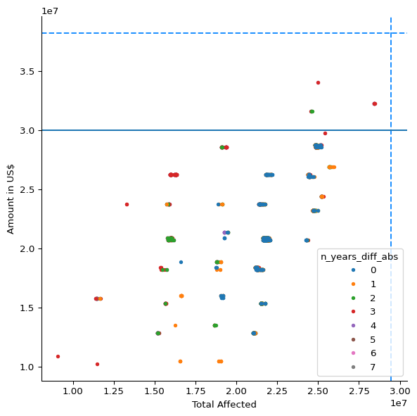
Select trigger combinations with exactly 2 years difference between forecast and observational triggers, and high CERF funding amounts.
### Filter for Two-Year Difference Combinations
df_twoyears = df_metrics_lowest[
    (df_metrics_lowest["n_years_diff_abs"] == 2)
    & (df_metrics_lowest["Amount in US$"] >= 3.0e7)
]df_twoyears| Total Affected | Total Deaths | Total Damage, Adjusted ('000 US$) | Amount in US$ | cerf | fcast_wind | fcast_rain_col | fcast_rain_thresh | obsv_wind | obsv_rain_col | obsv_rain_thresh | n_years_fcast | n_years_obsv | n_years_diff | n_years_diff_abs | n_years_total | |
|---|---|---|---|---|---|---|---|---|---|---|---|---|---|---|---|---|
| 312998 | 24602062.0 | 52.0 | 8142214.0 | 31582777.0 | 5.0 | 75.0 | mean | 69.391884 | 105.0 | q80_obsv | 96.217003 | 4 | 6 | -2 | 2 | 10 |
| 191213 | 24647558.0 | 53.0 | 8142214.0 | 31582777.0 | 5.0 | 35.0 | mean | 69.391884 | 105.0 | q80_obsv | 96.217003 | 4 | 6 | -2 | 2 | 10 |
| 191235 | 24602062.0 | 52.0 | 8142214.0 | 31582777.0 | 5.0 | 35.0 | mean | 71.266540 | 105.0 | q80_obsv | 96.217003 | 4 | 6 | -2 | 2 | 10 |
plot_selected_threshs(312998)(<Figure size 2800x1400 with 2 Axes>,
array([<Axes: title={'center': 'Action (forecast)'}, xlabel='\nMax. wind speed while in ZMA (knots)', ylabel='Two-day rainfall, mean over whole country (mm)'>,
<Axes: title={'center': 'Observational'}, xlabel='\nMax. wind speed while in ZMA (knots)', ylabel='Two-day rainfall, 80th quantile over whole country (mm)'>],
dtype=object))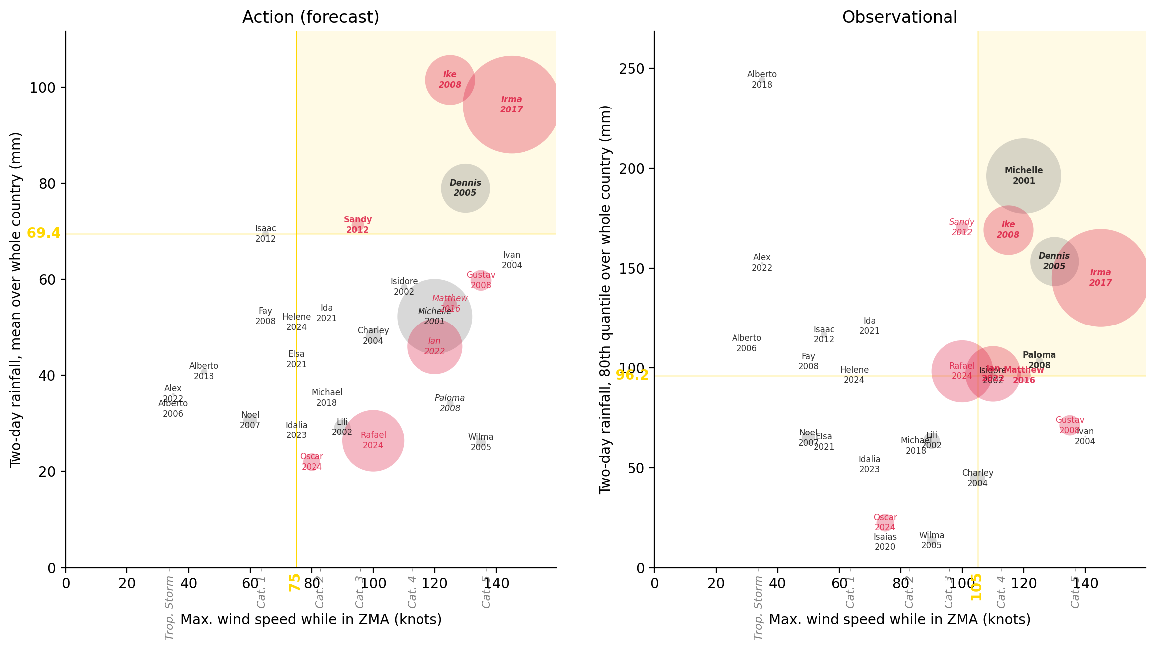
disp_selected_threshs(312998)| Action | Obsv. | CERF | Total Affected | |
|---|---|---|---|---|
| Storm | ||||
| Irma 2017 | Trig. | Trig. | Yes | 10,000,000 |
| Michelle 2001 | No trig. | Trig. | pre- | 5,900,012 |
| Rafael 2024 | No trig. | No trig. | Yes | 4,000,000 |
| Ian 2022 | No trig. | Trig. | Yes | 3,200,000 |
| Ike 2008 | Trig. | Trig. | Yes | 2,600,000 |
| Dennis 2005 | Trig. | Trig. | pre- | 2,500,000 |
| Gustav 2008 | No trig. | No trig. | Yes | 450,019 |
| Oscar 2024 | No trig. | No trig. | Yes | 320,000 |
| Lili 2002 | No trig. | No trig. | pre- | 281,470 |
| Charley 2004 | No trig. | No trig. | pre- | 244,005 |
| Noel 2007 | No trig. | No trig. | No | 192,488 |
| Matthew 2016 | No trig. | Trig. | Yes | 190,000 |
| Sandy 2012 | Trig. | No trig. | Yes | 162,605 |
| Wilma 2005 | No trig. | No trig. | pre- | 100,000 |
| Paloma 2008 | No trig. | Trig. | No | 49,445 |
| Isaac 2012 | No trig. | No trig. | No | 45,496 |
| Isidore 2002 | No trig. | No trig. | pre- | 42,500 |
| Alberto 2018 | No trig. | No trig. | No | 40,000 |
| Alex 2022 | No trig. | No trig. | No | 6,780 |
| Ivan 2004 | No trig. | No trig. | pre- | 3,245 |
| Michael 2018 | No trig. | No trig. | No | 540 |
| Isaias 2020 | No trig. | No trig. | No | 500 |
| Alberto 2006 | No trig. | No trig. | No | 268 |
| Ida 2021 | No trig. | No trig. | No | 0 |
| Elsa 2021 | No trig. | No trig. | No | 0 |
| Idalia 2023 | No trig. | No trig. | No | 0 |
| Helene 2024 | No trig. | No trig. | No | 0 |
| Dean 2007 | No trig. | No trig. | No | 0 |
| Fay 2008 | No trig. | No trig. | No | 0 |
Small cluster with second-best total impact (option 4 in slides)
fig, ax = plot_thresh_scatter(
    "Total Affected", "Amount in US$", "n_years_diff_abs"
)
ax.axvline(2.55e7)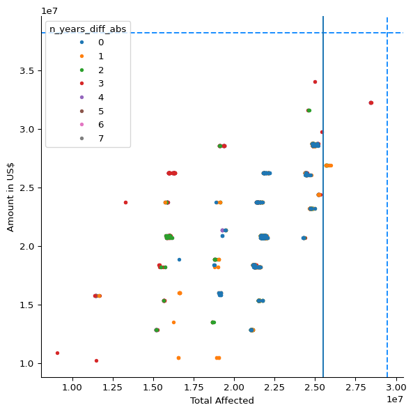
df_oneyear = df_metrics_lowest[
    (df_metrics_lowest["Total Affected"] >= 2.55e7)
    & (df_metrics_lowest["n_years_diff_abs"] == 1)
]df_oneyear| Total Affected | Total Deaths | Total Damage, Adjusted ('000 US$) | Amount in US$ | cerf | fcast_wind | fcast_rain_col | fcast_rain_thresh | obsv_wind | obsv_rain_col | obsv_rain_thresh | n_years_fcast | n_years_obsv | n_years_diff | n_years_diff_abs | n_years_total | |
|---|---|---|---|---|---|---|---|---|---|---|---|---|---|---|---|---|
| 201091 | 25710822.0 | 50.0 | 8073174.0 | 26889626.0 | 5.0 | 35.0 | mean | 59.768433 | 75.0 | q80_obsv | 98.341003 | 5 | 6 | -1 | 1 | 11 |
| 201377 | 25710822.0 | 50.0 | 8073174.0 | 26889626.0 | 5.0 | 35.0 | q80 | 103.080360 | 75.0 | q80_obsv | 98.341003 | 5 | 6 | -1 | 1 | 11 |
| 111447 | 25909331.0 | 53.0 | 9622569.0 | 26889626.0 | 5.0 | 90.0 | q80 | 87.754250 | 75.0 | q80_obsv | 98.341003 | 5 | 6 | -1 | 1 | 11 |
| 60958 | 25665326.0 | 49.0 | 8073174.0 | 26889626.0 | 5.0 | 120.0 | q50 | 42.302090 | 75.0 | q80_obsv | 98.341003 | 5 | 6 | -1 | 1 | 11 |
| 322018 | 25665326.0 | 49.0 | 8073174.0 | 26889626.0 | 5.0 | 75.0 | q80 | 103.080360 | 75.0 | q80_obsv | 98.341003 | 5 | 6 | -1 | 1 | 11 |
| 321720 | 25665326.0 | 49.0 | 8073174.0 | 26889626.0 | 5.0 | 75.0 | mean | 59.768433 | 75.0 | q80_obsv | 98.341003 | 5 | 6 | -1 | 1 | 11 |
| 201331 | 25954827.0 | 54.0 | 9622569.0 | 26889626.0 | 5.0 | 35.0 | q80 | 96.462585 | 75.0 | q80_obsv | 98.341003 | 5 | 6 | -1 | 1 | 11 |
| 321972 | 25909331.0 | 53.0 | 9622569.0 | 26889626.0 | 5.0 | 75.0 | q80 | 96.462585 | 75.0 | q80_obsv | 98.341003 | 5 | 6 | -1 | 1 | 11 |
plot_selected_threshs(321972)(<Figure size 2800x1400 with 2 Axes>,
array([<Axes: title={'center': 'Action (forecast)'}, xlabel='\nMax. wind speed while in ZMA (knots)', ylabel='Two-day rainfall, 80th quantile over whole country (mm)'>,
<Axes: title={'center': 'Observational'}, xlabel='\nMax. wind speed while in ZMA (knots)', ylabel='Two-day rainfall, 80th quantile over whole country (mm)'>],
dtype=object))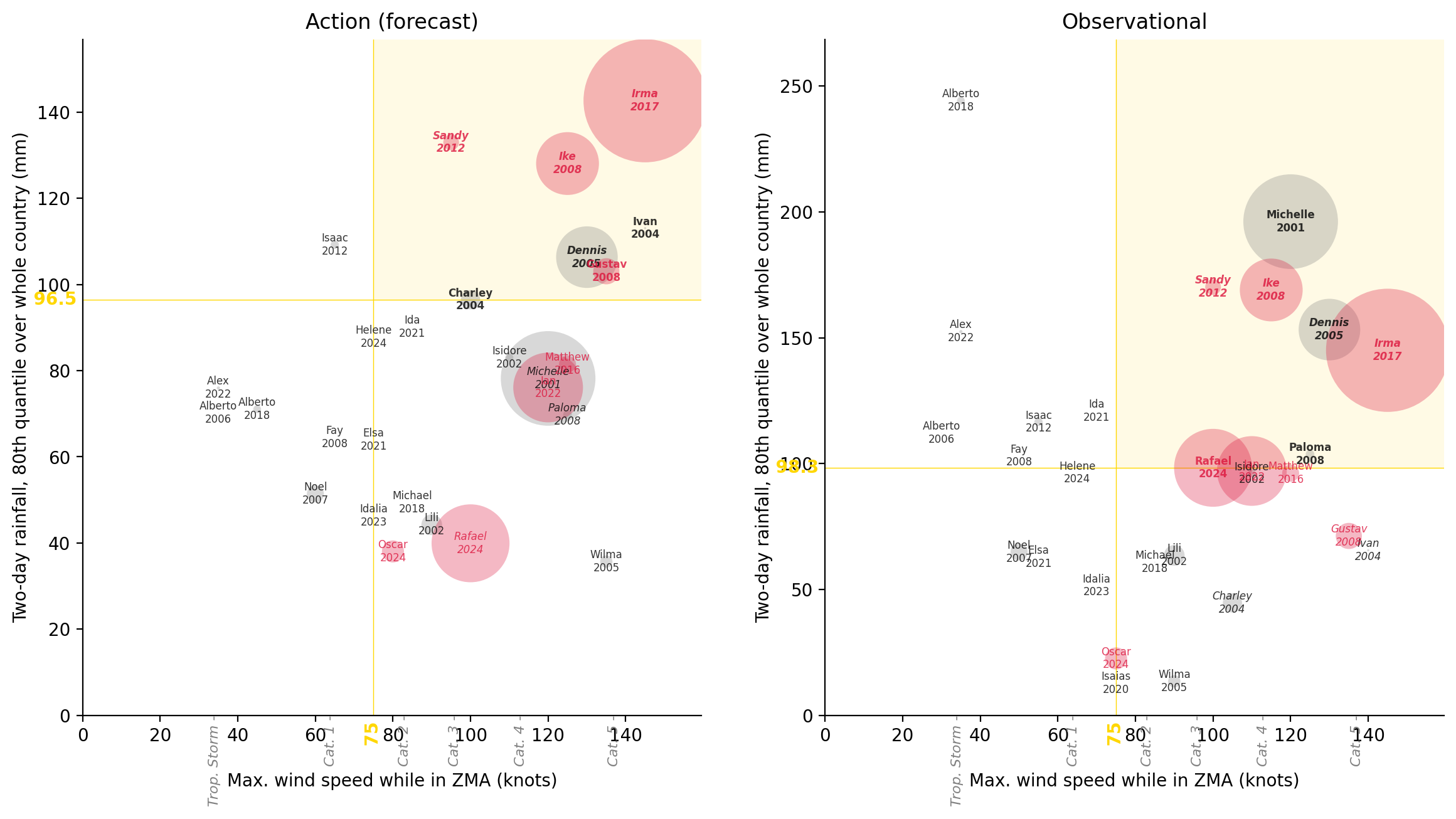
disp_selected_threshs(321972)| Action | Obsv. | CERF | Total Affected | |
|---|---|---|---|---|
| Storm | ||||
| Irma 2017 | Trig. | Trig. | Yes | 10,000,000 |
| Michelle 2001 | No trig. | Trig. | pre- | 5,900,012 |
| Rafael 2024 | No trig. | Trig. | Yes | 4,000,000 |
| Ian 2022 | No trig. | No trig. | Yes | 3,200,000 |
| Ike 2008 | Trig. | Trig. | Yes | 2,600,000 |
| Dennis 2005 | Trig. | Trig. | pre- | 2,500,000 |
| Gustav 2008 | Trig. | No trig. | Yes | 450,019 |
| Oscar 2024 | No trig. | No trig. | Yes | 320,000 |
| Lili 2002 | No trig. | No trig. | pre- | 281,470 |
| Charley 2004 | Trig. | No trig. | pre- | 244,005 |
| Noel 2007 | No trig. | No trig. | No | 192,488 |
| Matthew 2016 | No trig. | No trig. | Yes | 190,000 |
| Sandy 2012 | Trig. | Trig. | Yes | 162,605 |
| Wilma 2005 | No trig. | No trig. | pre- | 100,000 |
| Paloma 2008 | No trig. | Trig. | No | 49,445 |
| Isaac 2012 | No trig. | No trig. | No | 45,496 |
| Isidore 2002 | No trig. | No trig. | pre- | 42,500 |
| Alberto 2018 | No trig. | No trig. | No | 40,000 |
| Alex 2022 | No trig. | No trig. | No | 6,780 |
| Ivan 2004 | Trig. | No trig. | pre- | 3,245 |
| Michael 2018 | No trig. | No trig. | No | 540 |
| Isaias 2020 | No trig. | No trig. | No | 500 |
| Alberto 2006 | No trig. | No trig. | No | 268 |
| Ida 2021 | No trig. | No trig. | No | 0 |
| Elsa 2021 | No trig. | No trig. | No | 0 |
| Idalia 2023 | No trig. | No trig. | No | 0 |
| Helene 2024 | No trig. | No trig. | No | 0 |
| Dean 2007 | No trig. | No trig. | No | 0 |
| Fay 2008 | No trig. | No trig. | No | 0 |
Looking at how we can tilt probability even more towards forecast - basically just variants of option 1
fig, ax = plot_thresh_scatter(
    "Total Affected",
    "Amount in US$",
    "n_years_diff",
    fcast_pref_only=True,
    zorder_rev=False,
)
ax.axhline(2.7e7)
ax.axvline(2.3e7)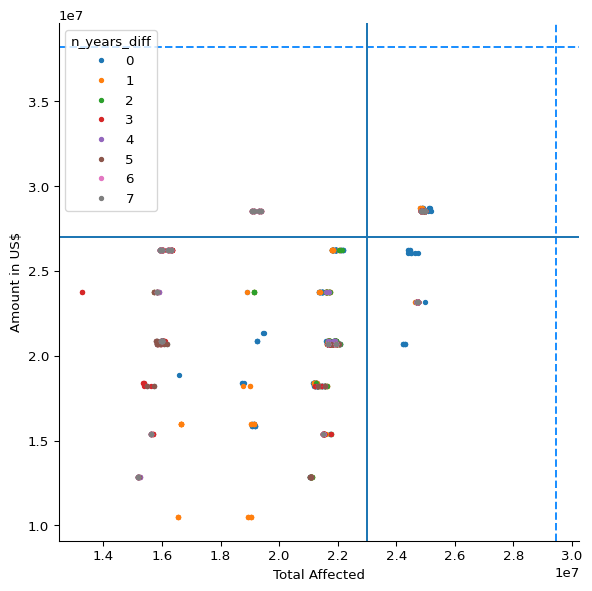
df_fcast_pref = df_metrics_lowest[
    (df_metrics_lowest["Total Affected"] >= 2.3e7)
    & (df_metrics_lowest["Amount in US$"] >= 2.7e7)
    & (df_metrics_lowest["n_years_diff"] >= 0)
]df_fcast_pref| Total Affected | Total Deaths | Total Damage, Adjusted ('000 US$) | Amount in US$ | cerf | fcast_wind | fcast_rain_col | fcast_rain_thresh | obsv_wind | obsv_rain_col | obsv_rain_thresh | n_years_fcast | n_years_obsv | n_years_diff | n_years_diff_abs | n_years_total | |
|---|---|---|---|---|---|---|---|---|---|---|---|---|---|---|---|---|
| 22746 | 24843276.0 | 41.0 | 11268506.0 | 28547455.0 | 5.0 | 120.0 | q80 | 70.166730 | 130.0 | q50_obsv | 2.44 | 7 | 4 | 3 | 3 | 11 |
| 38993 | 24992721.0 | 45.0 | 12317493.0 | 28547455.0 | 5.0 | 120.0 | mean | 21.936502 | 115.0 | q50_obsv | 2.44 | 7 | 6 | 1 | 1 | 13 |
| 44003 | 24992721.0 | 45.0 | 12317493.0 | 28547455.0 | 5.0 | 120.0 | q95 | 67.368840 | 115.0 | q50_obsv | 2.44 | 7 | 6 | 1 | 1 | 13 |
| 39109 | 24892721.0 | 41.0 | 11268506.0 | 28547455.0 | 5.0 | 120.0 | mean | 26.405380 | 115.0 | q50_obsv | 2.44 | 7 | 6 | 1 | 1 | 13 |
| 42119 | 24892721.0 | 41.0 | 11268506.0 | 28547455.0 | 5.0 | 120.0 | q80 | 38.042336 | 115.0 | q50_obsv | 2.44 | 7 | 6 | 1 | 1 | 13 |
| ... | ... | ... | ... | ... | ... | ... | ... | ... | ... | ... | ... | ... | ... | ... | ... | ... |
| 25792 | 24992721.0 | 45.0 | 12317493.0 | 28547455.0 | 5.0 | 120.0 | q95 | 67.368840 | 30.0 | q95_obsv | NaN | 7 | 0 | 7 | 7 | 7 |
| 25421 | 24992721.0 | 45.0 | 12317493.0 | 28547455.0 | 5.0 | 120.0 | q50 | 7.418959 | 30.0 | q80_obsv | NaN | 7 | 0 | 7 | 7 | 7 |
| 25422 | 24992721.0 | 45.0 | 12317493.0 | 28547455.0 | 5.0 | 120.0 | q50 | 7.418959 | 30.0 | q95_obsv | NaN | 7 | 0 | 7 | 7 | 7 |
| 25202 | 24992721.0 | 45.0 | 12317493.0 | 28547455.0 | 5.0 | 120.0 | mean | 21.936502 | 30.0 | q80_obsv | NaN | 7 | 0 | 7 | 7 | 7 |
| 25203 | 24992721.0 | 45.0 | 12317493.0 | 28547455.0 | 5.0 | 120.0 | mean | 21.936502 | 30.0 | q95_obsv | NaN | 7 | 0 | 7 | 7 | 7 |
160 rows × 16 columns
df_fcast_only = df_fcast_pref[df_fcast_pref["n_years_diff"] == 0]df_fcast_only| Total Affected | Total Deaths | Total Damage, Adjusted ('000 US$) | Amount in US$ | cerf | fcast_wind | fcast_rain_col | fcast_rain_thresh | obsv_wind | obsv_rain_col | obsv_rain_thresh | n_years_fcast | n_years_obsv | n_years_diff | n_years_diff_abs | n_years_total | |
|---|---|---|---|---|---|---|---|---|---|---|---|---|---|---|---|---|
| 71389 | 24843276.0 | 41.0 | 11268506.0 | 28547455.0 | 5.0 | 110.0 | q95 | 143.712340 | 105.0 | q50_obsv | 45.957497 | 5 | 5 | 0 | 0 | 10 |
| 119458 | 25087281.0 | 45.0 | 12817901.0 | 28547455.0 | 5.0 | 100.0 | q95 | 143.712340 | 105.0 | q50_obsv | 45.957497 | 5 | 5 | 0 | 0 | 10 |
| 119486 | 25187281.0 | 49.0 | 13866888.0 | 28547455.0 | 5.0 | 100.0 | q95 | 143.409800 | 105.0 | q50_obsv | 45.957497 | 5 | 5 | 0 | 0 | 10 |
| 71417 | 24943276.0 | 45.0 | 12317493.0 | 28547455.0 | 5.0 | 110.0 | q95 | 143.409800 | 105.0 | q50_obsv | 45.957497 | 5 | 5 | 0 | 0 | 10 |
| 60832 | 24865326.0 | 52.0 | 8098174.0 | 28717472.0 | 5.0 | 120.0 | q50 | 26.483074 | 75.0 | q50_obsv | 45.957497 | 6 | 6 | 0 | 0 | 12 |
| 60935 | 24815881.0 | 52.0 | 8098174.0 | 28717472.0 | 5.0 | 120.0 | q50 | 28.462177 | 75.0 | q50_obsv | 45.957497 | 6 | 6 | 0 | 0 | 12 |
| 191429 | 25154827.0 | 57.0 | 9647569.0 | 28717472.0 | 5.0 | 35.0 | q80 | 96.462585 | 105.0 | q80_obsv | 96.369003 | 5 | 5 | 0 | 0 | 10 |
| 98070 | 25109331.0 | 56.0 | 9647569.0 | 28717472.0 | 5.0 | 90.0 | q80 | 87.754250 | 105.0 | q80_obsv | 96.369003 | 5 | 5 | 0 | 0 | 10 |
| 313372 | 24865326.0 | 52.0 | 8098174.0 | 28717472.0 | 5.0 | 75.0 | q80 | 103.080360 | 105.0 | q80_obsv | 96.369003 | 5 | 5 | 0 | 0 | 10 |
| 191479 | 24910822.0 | 53.0 | 8098174.0 | 28717472.0 | 5.0 | 35.0 | q80 | 103.080360 | 105.0 | q80_obsv | 96.369003 | 5 | 5 | 0 | 0 | 10 |
| 312969 | 24865326.0 | 52.0 | 8098174.0 | 28717472.0 | 5.0 | 75.0 | mean | 59.768433 | 105.0 | q80_obsv | 96.369003 | 5 | 5 | 0 | 0 | 10 |
| 313322 | 25109331.0 | 56.0 | 9647569.0 | 28717472.0 | 5.0 | 75.0 | q80 | 96.462585 | 105.0 | q80_obsv | 96.369003 | 5 | 5 | 0 | 0 | 10 |
| 191184 | 24910822.0 | 53.0 | 8098174.0 | 28717472.0 | 5.0 | 35.0 | mean | 59.768433 | 105.0 | q80_obsv | 96.369003 | 5 | 5 | 0 | 0 | 10 |
plot_selected_threshs(25477) # not sure if worth leaving in book.(<Figure size 2800x1400 with 2 Axes>,
array([<Axes: title={'center': 'Action (forecast)'}, xlabel='\nMax. wind speed while in ZMA (knots)', ylabel='Two-day rainfall, 80th quantile over whole country (mm)'>,
<Axes: title={'center': 'Observational'}, xlabel='\nMax. wind speed while in ZMA (knots)', ylabel='Two-day rainfall, 80th quantile over whole country (mm)'>],
dtype=object))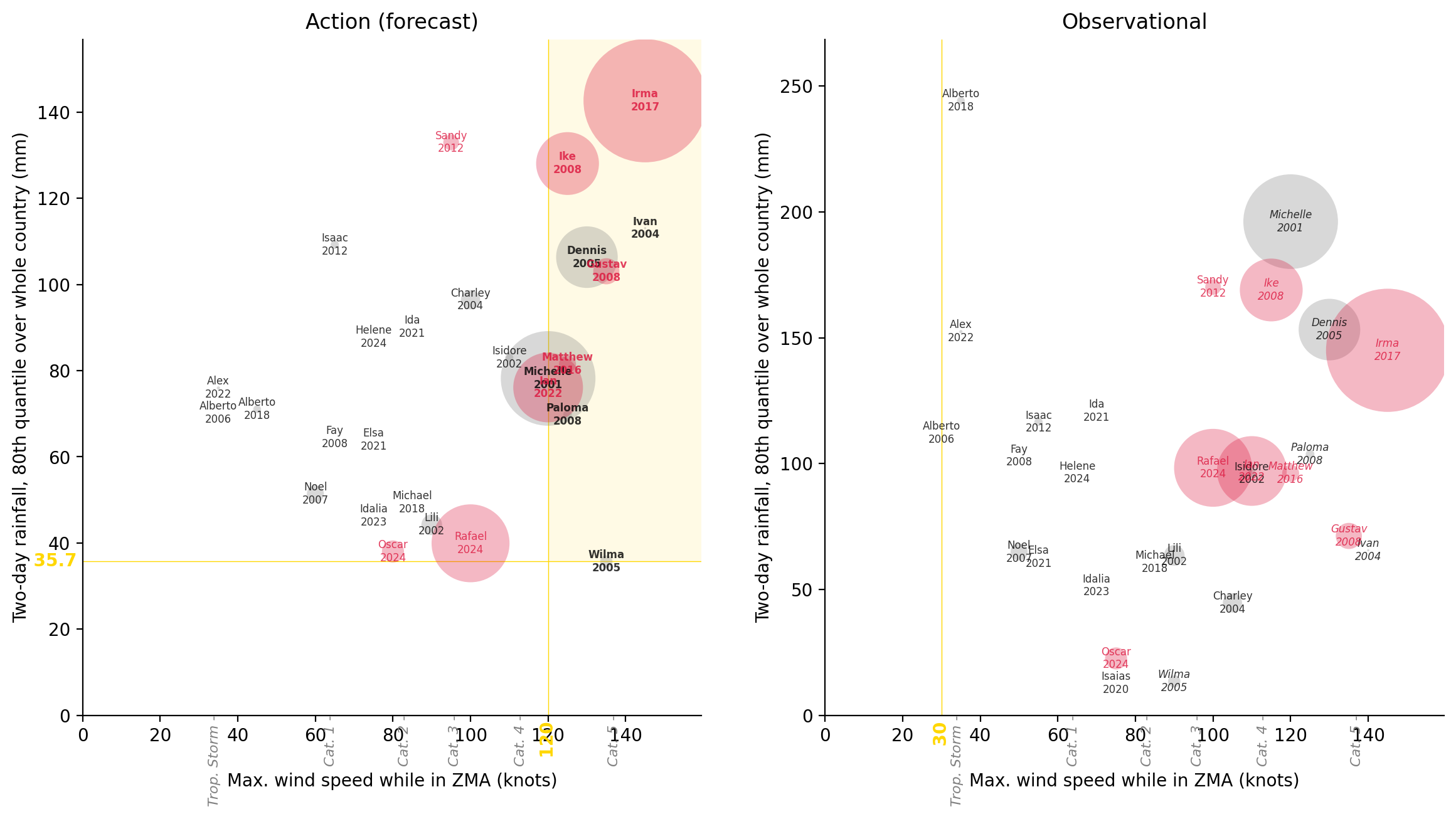
Keeping only options with same rainfall aggregation, and same windspeed across forecast and observational
df_simplified = df_metrics_lowest[
    (
        df_metrics_lowest["fcast_rain_col"]
        == df_metrics_lowest["obsv_rain_col"].str.removesuffix("_obsv")
    )
    & (df_metrics_lowest["fcast_wind"] == df_metrics_lowest["obsv_wind"])
]df_metrics_lowest[
(df_metrics_lowest["fcast_wind"] == df_metrics_lowest["obsv_wind"])
].sort_values("Total Affected", ascending=False)| Total Affected | Total Deaths | Total Damage, Adjusted ('000 US$) | Amount in US$ | cerf | fcast_wind | fcast_rain_col | fcast_rain_thresh | obsv_wind | obsv_rain_col | obsv_rain_thresh | n_years_fcast | n_years_obsv | n_years_diff | n_years_diff_abs | n_years_total | |
|---|---|---|---|---|---|---|---|---|---|---|---|---|---|---|---|---|
| 321743 | 28412062.0 | 52.0 | 4971882.0 | 32229929.0 | 5.0 | 75.0 | mean | 69.391884 | 75.0 | q80_obsv | 96.369003 | 4 | 7 | -3 | 3 | 11 |
| 321926 | 28412062.0 | 52.0 | 4971882.0 | 32229929.0 | 5.0 | 75.0 | q50 | 65.069570 | 75.0 | q80_obsv | 96.369003 | 3 | 7 | -4 | 4 | 10 |
| 321972 | 25909331.0 | 53.0 | 9622569.0 | 26889626.0 | 5.0 | 75.0 | q80 | 96.462585 | 75.0 | q80_obsv | 98.341003 | 5 | 6 | -1 | 1 | 11 |
| 322018 | 25665326.0 | 49.0 | 8073174.0 | 26889626.0 | 5.0 | 75.0 | q80 | 103.080360 | 75.0 | q80_obsv | 98.341003 | 5 | 6 | -1 | 1 | 11 |
| 321720 | 25665326.0 | 49.0 | 8073174.0 | 26889626.0 | 5.0 | 75.0 | mean | 59.768433 | 75.0 | q80_obsv | 98.341003 | 5 | 6 | -1 | 1 | 11 |
| 321846 | 25215307.0 | 49.0 | 5256761.0 | 24402195.0 | 4.0 | 75.0 | q50 | 61.708008 | 75.0 | q80_obsv | 98.341003 | 4 | 6 | -2 | 2 | 10 |
| 321994 | 25215307.0 | 49.0 | 5256761.0 | 24402195.0 | 4.0 | 75.0 | q80 | 106.357285 | 75.0 | q80_obsv | 98.341003 | 5 | 6 | -1 | 1 | 11 |
| 321679 | 25215307.0 | 49.0 | 5256761.0 | 24402195.0 | 4.0 | 75.0 | mean | 63.864970 | 75.0 | q80_obsv | 98.341003 | 5 | 6 | -1 | 1 | 11 |
| 321923 | 25136606.0 | 55.0 | 7863137.0 | 28717472.0 | 5.0 | 75.0 | q50 | 65.069570 | 75.0 | q50_obsv | 35.949997 | 3 | 7 | -4 | 4 | 10 |
| 321740 | 25136606.0 | 55.0 | 7863137.0 | 28717472.0 | 5.0 | 75.0 | mean | 69.391884 | 75.0 | q50_obsv | 35.949997 | 4 | 7 | -3 | 3 | 11 |
| 321970 | 25059886.0 | 56.0 | 9647569.0 | 28717472.0 | 5.0 | 75.0 | q80 | 96.462585 | 75.0 | q50_obsv | 45.957497 | 5 | 6 | -1 | 1 | 11 |
| 321924 | 24855136.0 | 52.0 | 7825716.0 | 28717472.0 | 5.0 | 75.0 | q50 | 65.069570 | 75.0 | q50_obsv | 38.012497 | 3 | 7 | -4 | 4 | 10 |
| 321741 | 24855136.0 | 52.0 | 7825716.0 | 28717472.0 | 5.0 | 75.0 | mean | 69.391884 | 75.0 | q50_obsv | 38.012497 | 4 | 7 | -3 | 3 | 11 |
| 321718 | 24815881.0 | 52.0 | 8098174.0 | 28717472.0 | 5.0 | 75.0 | mean | 59.768433 | 75.0 | q50_obsv | 45.957497 | 5 | 6 | -1 | 1 | 11 |
| 321844 | 24815881.0 | 52.0 | 8098174.0 | 28717472.0 | 5.0 | 75.0 | q50 | 61.708008 | 75.0 | q50_obsv | 45.957497 | 4 | 6 | -2 | 2 | 10 |
| 322016 | 24815881.0 | 52.0 | 8098174.0 | 28717472.0 | 5.0 | 75.0 | q80 | 103.080360 | 75.0 | q50_obsv | 45.957497 | 5 | 6 | -1 | 1 | 11 |
| 321920 | 24454562.0 | 52.0 | 5009303.0 | 26230041.0 | 4.0 | 75.0 | q50 | 65.069570 | 75.0 | mean_obsv | 51.583454 | 3 | 7 | -4 | 4 | 10 |
| 321737 | 24454562.0 | 52.0 | 5009303.0 | 26230041.0 | 4.0 | 75.0 | mean | 69.391884 | 75.0 | mean_obsv | 51.583454 | 4 | 7 | -3 | 3 | 11 |
| 321678 | 24365862.0 | 52.0 | 5281761.0 | 26230041.0 | 4.0 | 75.0 | mean | 63.864970 | 75.0 | q50_obsv | 47.079998 | 5 | 6 | -1 | 1 | 11 |
| 321845 | 24365862.0 | 52.0 | 5281761.0 | 26230041.0 | 4.0 | 75.0 | q50 | 61.708008 | 75.0 | q50_obsv | 47.079998 | 4 | 6 | -2 | 2 | 10 |
| 321993 | 24365862.0 | 52.0 | 5281761.0 | 26230041.0 | 4.0 | 75.0 | q80 | 106.357285 | 75.0 | q50_obsv | 47.079998 | 5 | 6 | -1 | 1 | 11 |
| 321965 | 21951831.0 | 53.0 | 9659990.0 | 20889738.0 | 4.0 | 75.0 | q80 | 96.462585 | 75.0 | mean_obsv | 55.230145 | 5 | 6 | -1 | 1 | 11 |
| 321967 | 21902386.0 | 53.0 | 9659990.0 | 20889738.0 | 4.0 | 75.0 | q80 | 96.462585 | 75.0 | mean_obsv | 74.488056 | 5 | 6 | -1 | 1 | 11 |
| 321644 | 21707826.0 | 49.0 | 8110595.0 | 20889738.0 | 4.0 | 75.0 | mean | 58.365227 | 75.0 | mean_obsv | 55.230145 | 6 | 6 | 0 | 0 | 12 |
| 322011 | 21707826.0 | 49.0 | 8110595.0 | 20889738.0 | 4.0 | 75.0 | q80 | 103.080360 | 75.0 | mean_obsv | 55.230145 | 5 | 6 | -1 | 1 | 11 |
| 321660 | 21707826.0 | 49.0 | 8110595.0 | 20889738.0 | 4.0 | 75.0 | mean | 58.365227 | 75.0 | q80_obsv | 103.079987 | 6 | 5 | 1 | 1 | 11 |
| 321655 | 21658381.0 | 49.0 | 8110595.0 | 20889738.0 | 4.0 | 75.0 | mean | 58.365227 | 75.0 | q50_obsv | 58.065002 | 6 | 5 | 1 | 1 | 11 |
| 321647 | 21658381.0 | 49.0 | 8110595.0 | 20889738.0 | 4.0 | 75.0 | mean | 58.365227 | 75.0 | mean_obsv | 74.488056 | 6 | 6 | 0 | 0 | 12 |
| 322013 | 21658381.0 | 49.0 | 8110595.0 | 20889738.0 | 4.0 | 75.0 | q80 | 103.080360 | 75.0 | mean_obsv | 74.488056 | 5 | 6 | -1 | 1 | 11 |
| 321659 | 21658381.0 | 49.0 | 8110595.0 | 20889738.0 | 4.0 | 75.0 | mean | 58.365227 | 75.0 | q80_obsv | 112.148994 | 6 | 5 | 1 | 1 | 11 |
| 321810 | 21495776.0 | 38.0 | 8110595.0 | 15366985.0 | 3.0 | 75.0 | q50 | 42.807594 | 75.0 | q50_obsv | 60.637505 | 7 | 4 | 3 | 3 | 11 |
| 321747 | 21444562.0 | 49.0 | 8154635.0 | 23755043.0 | 4.0 | 75.0 | mean | 69.391884 | 75.0 | q95_obsv | 186.113480 | 4 | 7 | -3 | 3 | 11 |
| 321930 | 21444562.0 | 49.0 | 8154635.0 | 23755043.0 | 4.0 | 75.0 | q50 | 65.069570 | 75.0 | q95_obsv | 186.113480 | 3 | 7 | -4 | 4 | 10 |
| 321672 | 21257807.0 | 49.0 | 5294182.0 | 18402307.0 | 3.0 | 75.0 | mean | 63.864970 | 75.0 | mean_obsv | 55.230145 | 5 | 6 | -1 | 1 | 11 |
| 321829 | 21257807.0 | 49.0 | 5294182.0 | 18402307.0 | 3.0 | 75.0 | q50 | 55.458720 | 75.0 | q80_obsv | 103.079987 | 5 | 5 | 0 | 0 | 10 |
| 321821 | 21257807.0 | 49.0 | 5294182.0 | 18402307.0 | 3.0 | 75.0 | q50 | 55.458720 | 75.0 | mean_obsv | 55.230145 | 5 | 6 | -1 | 1 | 11 |
| 321987 | 21257807.0 | 49.0 | 5294182.0 | 18402307.0 | 3.0 | 75.0 | q80 | 106.357285 | 75.0 | mean_obsv | 55.230145 | 5 | 6 | -1 | 1 | 11 |
| 321674 | 21208362.0 | 49.0 | 5294182.0 | 18402307.0 | 3.0 | 75.0 | mean | 63.864970 | 75.0 | mean_obsv | 74.488056 | 5 | 6 | -1 | 1 | 11 |
| 321989 | 21208362.0 | 49.0 | 5294182.0 | 18402307.0 | 3.0 | 75.0 | q80 | 106.357285 | 75.0 | mean_obsv | 74.488056 | 5 | 6 | -1 | 1 | 11 |
| 321823 | 21208362.0 | 49.0 | 5294182.0 | 18402307.0 | 3.0 | 75.0 | q50 | 55.458720 | 75.0 | mean_obsv | 74.488056 | 5 | 6 | -1 | 1 | 11 |
| 321826 | 21208362.0 | 49.0 | 5294182.0 | 18402307.0 | 3.0 | 75.0 | q50 | 55.458720 | 75.0 | q50_obsv | 58.065002 | 5 | 5 | 0 | 0 | 10 |
| 321828 | 21208362.0 | 49.0 | 5294182.0 | 18402307.0 | 3.0 | 75.0 | q50 | 55.458720 | 75.0 | q80_obsv | 112.148994 | 5 | 5 | 0 | 0 | 10 |
| 321960 | 21045757.0 | 38.0 | 5294182.0 | 12879554.0 | 2.0 | 75.0 | q50 | 47.932934 | 75.0 | q50_obsv | 60.637505 | 6 | 4 | 2 | 2 | 10 |
plot_thresh_scatter(
    "Total Affected",
    "Amount in US$",
    color="n_years_diff_abs",
    zero_intercept=True,
)
(<Figure size 672x672 with 1 Axes>,
<Axes: xlabel='Total Affected', ylabel='Amount in US$'>)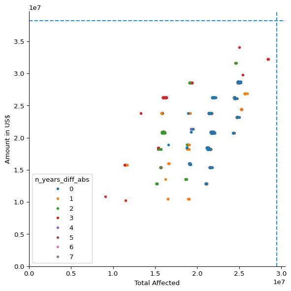
plot_thresh_scatter(
    "Total Affected",
    "Amount in US$",
    color="n_years_diff_abs",
    same_wind=True,
    zero_intercept=True,
)
(<Figure size 672x672 with 1 Axes>,
<Axes: xlabel='Total Affected', ylabel='Amount in US$'>)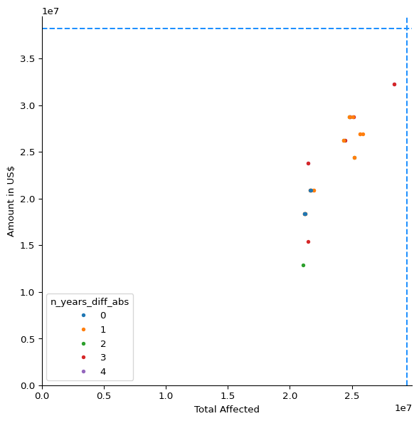
plot_thresh_scatter(
    "Total Affected",
    "Amount in US$",
    color="n_years_diff_abs",
    same_rain_col=True,
    zero_intercept=True,
)
(<Figure size 672x672 with 1 Axes>,
<Axes: xlabel='Total Affected', ylabel='Amount in US$'>)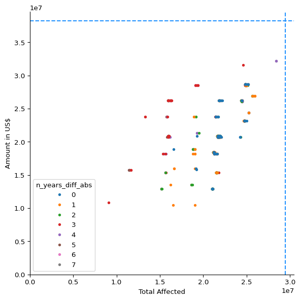
plot_thresh_scatter(
    "Total Affected",
    "Amount in US$",
    color="n_years_diff_abs",
    same_rain_col=True,
    same_wind=True,
    zero_intercept=True,
)
(<Figure size 672x672 with 1 Axes>,
<Axes: xlabel='Total Affected', ylabel='Amount in US$'>)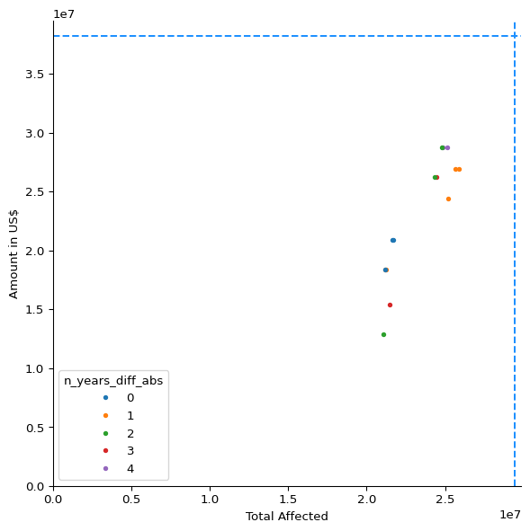
df_simplified.sort_values(
    ["Amount in US$", "Total Affected"],
    ascending=False,
)| Total Affected | Total Deaths | Total Damage, Adjusted ('000 US$) | Amount in US$ | cerf | fcast_wind | fcast_rain_col | fcast_rain_thresh | obsv_wind | obsv_rain_col | obsv_rain_thresh | n_years_fcast | n_years_obsv | n_years_diff | n_years_diff_abs | n_years_total | |
|---|---|---|---|---|---|---|---|---|---|---|---|---|---|---|---|---|
| 321923 | 25136606.0 | 55.0 | 7863137.0 | 28717472.0 | 5.0 | 75.0 | q50 | 65.069570 | 75.0 | q50_obsv | 35.949997 | 3 | 7 | -4 | 4 | 10 |
| 321924 | 24855136.0 | 52.0 | 7825716.0 | 28717472.0 | 5.0 | 75.0 | q50 | 65.069570 | 75.0 | q50_obsv | 38.012497 | 3 | 7 | -4 | 4 | 10 |
| 321844 | 24815881.0 | 52.0 | 8098174.0 | 28717472.0 | 5.0 | 75.0 | q50 | 61.708008 | 75.0 | q50_obsv | 45.957497 | 4 | 6 | -2 | 2 | 10 |
| 321972 | 25909331.0 | 53.0 | 9622569.0 | 26889626.0 | 5.0 | 75.0 | q80 | 96.462585 | 75.0 | q80_obsv | 98.341003 | 5 | 6 | -1 | 1 | 11 |
| 322018 | 25665326.0 | 49.0 | 8073174.0 | 26889626.0 | 5.0 | 75.0 | q80 | 103.080360 | 75.0 | q80_obsv | 98.341003 | 5 | 6 | -1 | 1 | 11 |
| 321737 | 24454562.0 | 52.0 | 5009303.0 | 26230041.0 | 4.0 | 75.0 | mean | 69.391884 | 75.0 | mean_obsv | 51.583454 | 4 | 7 | -3 | 3 | 11 |
| 321845 | 24365862.0 | 52.0 | 5281761.0 | 26230041.0 | 4.0 | 75.0 | q50 | 61.708008 | 75.0 | q50_obsv | 47.079998 | 4 | 6 | -2 | 2 | 10 |
| 321994 | 25215307.0 | 49.0 | 5256761.0 | 24402195.0 | 4.0 | 75.0 | q80 | 106.357285 | 75.0 | q80_obsv | 98.341003 | 5 | 6 | -1 | 1 | 11 |
| 321644 | 21707826.0 | 49.0 | 8110595.0 | 20889738.0 | 4.0 | 75.0 | mean | 58.365227 | 75.0 | mean_obsv | 55.230145 | 6 | 6 | 0 | 0 | 12 |
| 321647 | 21658381.0 | 49.0 | 8110595.0 | 20889738.0 | 4.0 | 75.0 | mean | 58.365227 | 75.0 | mean_obsv | 74.488056 | 6 | 6 | 0 | 0 | 12 |
| 321672 | 21257807.0 | 49.0 | 5294182.0 | 18402307.0 | 3.0 | 75.0 | mean | 63.864970 | 75.0 | mean_obsv | 55.230145 | 5 | 6 | -1 | 1 | 11 |
| 321826 | 21208362.0 | 49.0 | 5294182.0 | 18402307.0 | 3.0 | 75.0 | q50 | 55.458720 | 75.0 | q50_obsv | 58.065002 | 5 | 5 | 0 | 0 | 10 |
| 321674 | 21208362.0 | 49.0 | 5294182.0 | 18402307.0 | 3.0 | 75.0 | mean | 63.864970 | 75.0 | mean_obsv | 74.488056 | 5 | 6 | -1 | 1 | 11 |
| 321810 | 21495776.0 | 38.0 | 8110595.0 | 15366985.0 | 3.0 | 75.0 | q50 | 42.807594 | 75.0 | q50_obsv | 60.637505 | 7 | 4 | 3 | 3 | 11 |
| 321960 | 21045757.0 | 38.0 | 5294182.0 | 12879554.0 | 2.0 | 75.0 | q50 | 47.932934 | 75.0 | q50_obsv | 60.637505 | 6 | 4 | 2 | 2 | 10 |
plot_selected_threshs(321844)(<Figure size 2800x1400 with 2 Axes>,
array([<Axes: title={'center': 'Action (forecast)'}, xlabel='\nMax. wind speed while in ZMA (knots)', ylabel='Two-day rainfall, median over whole country (mm)'>,
<Axes: title={'center': 'Observational'}, xlabel='\nMax. wind speed while in ZMA (knots)', ylabel='Two-day rainfall, median over whole country (mm)'>],
dtype=object))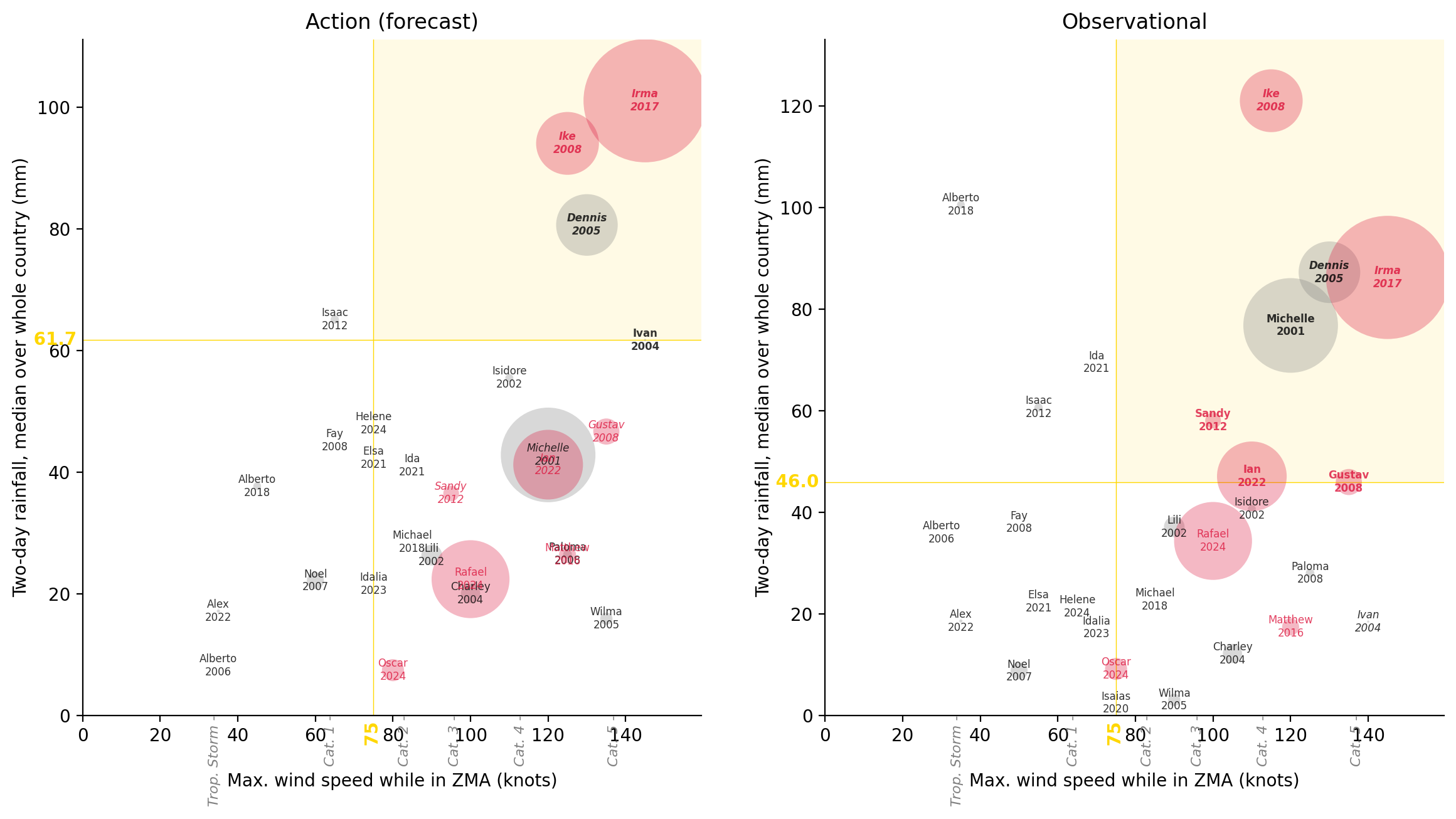
disp_selected_threshs(321844)| Action | Obsv. | CERF | Total Affected | |
|---|---|---|---|---|
| Storm | ||||
| Irma 2017 | Trig. | Trig. | Yes | 10,000,000 |
| Michelle 2001 | No trig. | Trig. | pre- | 5,900,012 |
| Rafael 2024 | No trig. | No trig. | Yes | 4,000,000 |
| Ian 2022 | No trig. | Trig. | Yes | 3,200,000 |
| Ike 2008 | Trig. | Trig. | Yes | 2,600,000 |
| Dennis 2005 | Trig. | Trig. | pre- | 2,500,000 |
| Gustav 2008 | No trig. | Trig. | Yes | 450,019 |
| Oscar 2024 | No trig. | No trig. | Yes | 320,000 |
| Lili 2002 | No trig. | No trig. | pre- | 281,470 |
| Charley 2004 | No trig. | No trig. | pre- | 244,005 |
| Noel 2007 | No trig. | No trig. | No | 192,488 |
| Matthew 2016 | No trig. | No trig. | Yes | 190,000 |
| Sandy 2012 | No trig. | Trig. | Yes | 162,605 |
| Wilma 2005 | No trig. | No trig. | pre- | 100,000 |
| Paloma 2008 | No trig. | No trig. | No | 49,445 |
| Isaac 2012 | No trig. | No trig. | No | 45,496 |
| Isidore 2002 | No trig. | No trig. | pre- | 42,500 |
| Alberto 2018 | No trig. | No trig. | No | 40,000 |
| Alex 2022 | No trig. | No trig. | No | 6,780 |
| Ivan 2004 | Trig. | No trig. | pre- | 3,245 |
| Michael 2018 | No trig. | No trig. | No | 540 |
| Isaias 2020 | No trig. | No trig. | No | 500 |
| Alberto 2006 | No trig. | No trig. | No | 268 |
| Ida 2021 | No trig. | No trig. | No | 0 |
| Elsa 2021 | No trig. | No trig. | No | 0 |
| Idalia 2023 | No trig. | No trig. | No | 0 |
| Helene 2024 | No trig. | No trig. | No | 0 |
| Dean 2007 | No trig. | No trig. | No | 0 |
| Fay 2008 | No trig. | No trig. | No | 0 |
df_metrics_lowest| Total Affected | Total Deaths | Total Damage, Adjusted ('000 US$) | Amount in US$ | cerf | fcast_wind | fcast_rain_col | fcast_rain_thresh | obsv_wind | obsv_rain_col | obsv_rain_thresh | n_years_fcast | n_years_obsv | n_years_diff | n_years_diff_abs | n_years_total | |
|---|---|---|---|---|---|---|---|---|---|---|---|---|---|---|---|---|
| 332720 | 24745221.0 | 41.0 | 8135595.0 | 23194719.0 | 4.0 | 80.0 | q50 | 41.205720 | 125.0 | q50_obsv | 2.44 | 7 | 4 | 3 | 3 | 11 |
| 198088 | 16341819.0 | 52.0 | 13714030.0 | 26242474.0 | 5.0 | 35.0 | q95 | 141.738710 | 125.0 | q50_obsv | 2.44 | 7 | 4 | 3 | 3 | 11 |
| 22746 | 24843276.0 | 41.0 | 11268506.0 | 28547455.0 | 5.0 | 120.0 | q80 | 70.166730 | 130.0 | q50_obsv | 2.44 | 7 | 4 | 3 | 3 | 11 |
| 82763 | 21735221.0 | 38.0 | 11280927.0 | 20719721.0 | 4.0 | 110.0 | q80 | 78.203220 | 115.0 | q50_obsv | 2.44 | 7 | 6 | 1 | 1 | 13 |
| 314406 | 21495776.0 | 38.0 | 8110595.0 | 15366985.0 | 3.0 | 75.0 | q50 | 42.807594 | 130.0 | q50_obsv | 2.44 | 7 | 4 | 3 | 3 | 11 |
| ... | ... | ... | ... | ... | ... | ... | ... | ... | ... | ... | ... | ... | ... | ... | ... | ... |
| 25202 | 24992721.0 | 45.0 | 12317493.0 | 28547455.0 | 5.0 | 120.0 | mean | 21.936502 | 30.0 | q80_obsv | NaN | 7 | 0 | 7 | 7 | 7 |
| 25203 | 24992721.0 | 45.0 | 12317493.0 | 28547455.0 | 5.0 | 120.0 | mean | 21.936502 | 30.0 | q95_obsv | NaN | 7 | 0 | 7 | 7 | 7 |
| 100940 | 16292374.0 | 52.0 | 13714030.0 | 26242474.0 | 5.0 | 90.0 | q95 | 140.547760 | 30.0 | mean_obsv | NaN | 7 | 0 | 7 | 7 | 7 |
| 100943 | 16292374.0 | 52.0 | 13714030.0 | 26242474.0 | 5.0 | 90.0 | q95 | 140.547760 | 30.0 | q80_obsv | NaN | 7 | 0 | 7 | 7 | 7 |
| 328878 | 24695776.0 | 41.0 | 8135595.0 | 23194719.0 | 4.0 | 80.0 | q50 | 41.205720 | 30.0 | q80_obsv | NaN | 7 | 0 | 7 | 7 | 7 |
2543 rows × 16 columns
Trigger combos that meet:
q50 and q80for stage in ["fcast", "obsv"]:
df_metrics_lowest[f"{stage}_cat"] = df_metrics_lowest[
f"{stage}_wind"
].apply(knots2cat)
df_metrics_lowest["cat_diff"] = (
df_metrics_lowest["fcast_cat"] - df_metrics_lowest["obsv_cat"]
)
df_metrics_lowest["min_cat"] = df_metrics_lowest[
["fcast_cat", "obsv_cat"]
].min(axis=1)df_metrics_reasonable = df_metrics_lowest[
(df_metrics_lowest["cat_diff"].isin([0, 1]))
& (df_metrics_lowest["min_cat"] >= 1)
& (
df_metrics_lowest["fcast_rain_col"]
== df_metrics_lowest["obsv_rain_col"].str.removesuffix("_obsv")
)
& (df_metrics_lowest["fcast_rain_col"].isin(["q50", "q80"]))
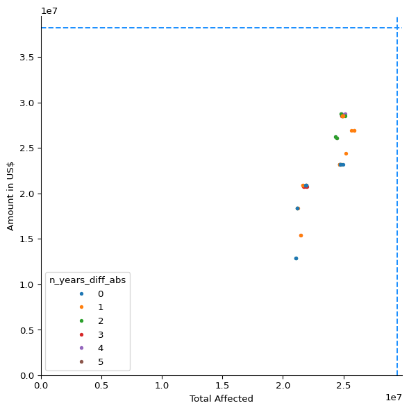
].copy()len(df_metrics_reasonable)59fig, ax = plot_thresh_scatter(
df=df_metrics_reasonable,
zero_intercept=True,
# color="n_years_diff",
# zorder_rev=False,
)
fig, ax = plot_thresh_scatter(
    df=df_metrics_reasonable,
    zero_intercept=True,
    # color="n_years_diff",
    # zorder_rev=False,
)
ax.axhline(2.8e7)
ax.axvline(2.55e7)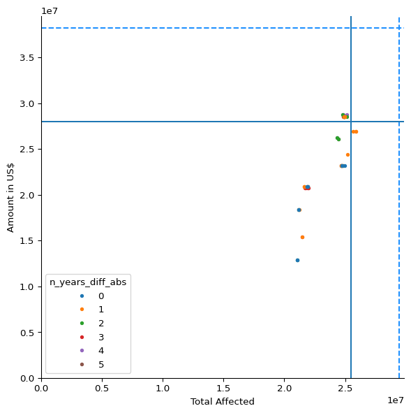
df_metrics_reasonable_bestcerf = df_metrics_reasonable[
    df_metrics_reasonable["Amount in US$"] >= 2.8e7
]df_metrics_reasonable_bestcerf[
df_metrics_reasonable_bestcerf["n_years_diff"] == 1
]| Total Affected | Total Deaths | Total Damage, Adjusted ('000 US$) | Amount in US$ | cerf | fcast_wind | fcast_rain_col | fcast_rain_thresh | obsv_wind | obsv_rain_col | obsv_rain_thresh | n_years_fcast | n_years_obsv | n_years_diff | n_years_diff_abs | n_years_total | fcast_cat | obsv_cat | cat_diff | min_cat | |
|---|---|---|---|---|---|---|---|---|---|---|---|---|---|---|---|---|---|---|---|---|
| 40495 | 24992721.0 | 45.0 | 12317493.0 | 28547455.0 | 5.0 | 120.0 | q50 | 7.418959 | 115.0 | q50_obsv | 2.440000 | 7 | 6 | 1 | 1 | 13 | 4 | 4 | 0 | 4 |
| 40206 | 24892721.0 | 41.0 | 11268506.0 | 28547455.0 | 5.0 | 120.0 | q50 | 17.138527 | 115.0 | q50_obsv | 2.440000 | 7 | 6 | 1 | 1 | 13 | 4 | 4 | 0 | 4 |
| 42148 | 24892721.0 | 41.0 | 11268506.0 | 28547455.0 | 5.0 | 120.0 | q80 | 38.042336 | 115.0 | q80_obsv | 12.709001 | 7 | 6 | 1 | 1 | 13 | 4 | 4 | 0 | 4 |
| 40872 | 24992721.0 | 45.0 | 12317493.0 | 28547455.0 | 5.0 | 120.0 | q80 | 35.698547 | 115.0 | q80_obsv | 12.709001 | 7 | 6 | 1 | 1 | 13 | 4 | 4 | 0 | 4 |
| 13724 | 24892721.0 | 41.0 | 11268506.0 | 28547455.0 | 5.0 | 120.0 | q80 | 38.042336 | 105.0 | q80_obsv | 96.217003 | 7 | 6 | 1 | 1 | 13 | 4 | 3 | 1 | 3 |
| 13136 | 24992721.0 | 45.0 | 12317493.0 | 28547455.0 | 5.0 | 120.0 | q80 | 35.698547 | 105.0 | q80_obsv | 96.217003 | 7 | 6 | 1 | 1 | 13 | 4 | 3 | 1 | 3 |
Maximizing CERF, taking closest to balanced (n_years_diff == 1), and lowest obsv wind threshold.
plot_selected_threshs(13136)(<Figure size 2800x1400 with 2 Axes>,
array([<Axes: title={'center': 'Action (forecast)'}, xlabel='\nMax. wind speed while in ZMA (knots)', ylabel='Two-day rainfall, 80th quantile over whole country (mm)'>,
<Axes: title={'center': 'Observational'}, xlabel='\nMax. wind speed while in ZMA (knots)', ylabel='Two-day rainfall, 80th quantile over whole country (mm)'>],
dtype=object))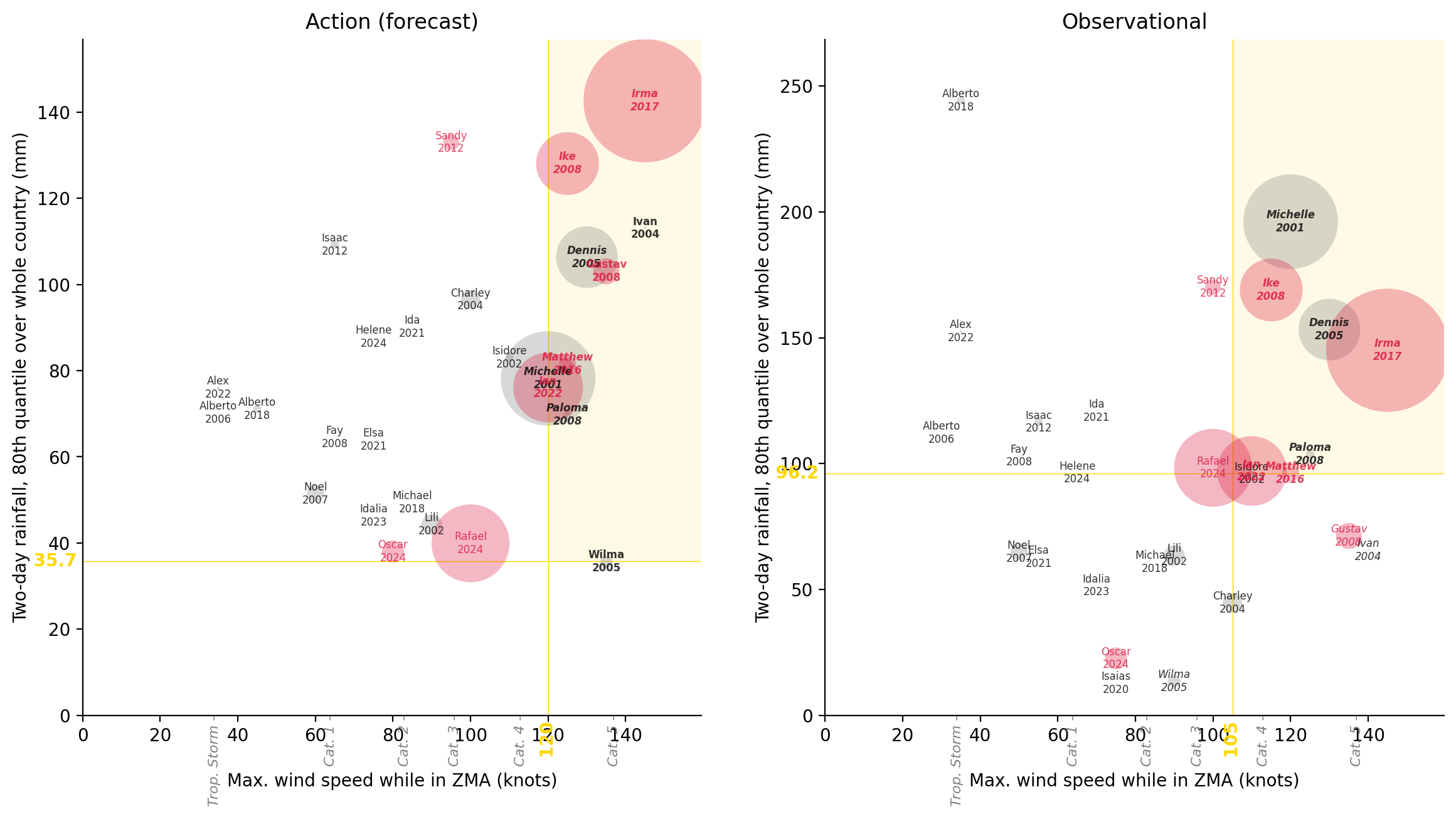
disp_selected_threshs(13136)| Action | Obsv. | CERF | Total Affected | |
|---|---|---|---|---|
| Storm | ||||
| Irma 2017 | Trig. | Trig. | Yes | 10,000,000 |
| Michelle 2001 | Trig. | Trig. | pre- | 5,900,012 |
| Rafael 2024 | No trig. | No trig. | Yes | 4,000,000 |
| Ian 2022 | Trig. | Trig. | Yes | 3,200,000 |
| Ike 2008 | Trig. | Trig. | Yes | 2,600,000 |
| Dennis 2005 | Trig. | Trig. | pre- | 2,500,000 |
| Gustav 2008 | Trig. | No trig. | Yes | 450,019 |
| Oscar 2024 | No trig. | No trig. | Yes | 320,000 |
| Lili 2002 | No trig. | No trig. | pre- | 281,470 |
| Charley 2004 | No trig. | No trig. | pre- | 244,005 |
| Noel 2007 | No trig. | No trig. | No | 192,488 |
| Matthew 2016 | Trig. | Trig. | Yes | 190,000 |
| Sandy 2012 | No trig. | No trig. | Yes | 162,605 |
| Wilma 2005 | Trig. | No trig. | pre- | 100,000 |
| Paloma 2008 | Trig. | Trig. | No | 49,445 |
| Isaac 2012 | No trig. | No trig. | No | 45,496 |
| Isidore 2002 | No trig. | No trig. | pre- | 42,500 |
| Alberto 2018 | No trig. | No trig. | No | 40,000 |
| Alex 2022 | No trig. | No trig. | No | 6,780 |
| Ivan 2004 | Trig. | No trig. | pre- | 3,245 |
| Michael 2018 | No trig. | No trig. | No | 540 |
| Isaias 2020 | No trig. | No trig. | No | 500 |
| Alberto 2006 | No trig. | No trig. | No | 268 |
| Ida 2021 | No trig. | No trig. | No | 0 |
| Elsa 2021 | No trig. | No trig. | No | 0 |
| Idalia 2023 | No trig. | No trig. | No | 0 |
| Helene 2024 | No trig. | No trig. | No | 0 |
| Dean 2007 | No trig. | No trig. | No | 0 |
| Fay 2008 | No trig. | No trig. | No | 0 |
Taking the maximum impact just ends up with option 4 again
df_metrics_reasonable_bestimpact = df_metrics_reasonable[
    df_metrics_reasonable["Total Affected"] >= 2.55e7
]df_metrics_reasonable_bestimpact| Total Affected | Total Deaths | Total Damage, Adjusted ('000 US$) | Amount in US$ | cerf | fcast_wind | fcast_rain_col | fcast_rain_thresh | obsv_wind | obsv_rain_col | obsv_rain_thresh | n_years_fcast | n_years_obsv | n_years_diff | n_years_diff_abs | n_years_total | fcast_cat | obsv_cat | cat_diff | min_cat | |
|---|---|---|---|---|---|---|---|---|---|---|---|---|---|---|---|---|---|---|---|---|
| 111447 | 25909331.0 | 53.0 | 9622569.0 | 26889626.0 | 5.0 | 90.0 | q80 | 87.754250 | 75.0 | q80_obsv | 98.341003 | 5 | 6 | -1 | 1 | 11 | 2 | 1 | 1 | 1 |
| 322018 | 25665326.0 | 49.0 | 8073174.0 | 26889626.0 | 5.0 | 75.0 | q80 | 103.080360 | 75.0 | q80_obsv | 98.341003 | 5 | 6 | -1 | 1 | 11 | 1 | 1 | 0 | 1 |
| 321972 | 25909331.0 | 53.0 | 9622569.0 | 26889626.0 | 5.0 | 75.0 | q80 | 96.462585 | 75.0 | q80_obsv | 98.341003 | 5 | 6 | -1 | 1 | 11 | 1 | 1 | 0 | 1 |
plot_selected_threshs(321972)(<Figure size 2800x1400 with 2 Axes>,
array([<Axes: title={'center': 'Action (forecast)'}, xlabel='\nMax. wind speed while in ZMA (knots)', ylabel='Two-day rainfall, 80th quantile over whole country (mm)'>,
<Axes: title={'center': 'Observational'}, xlabel='\nMax. wind speed while in ZMA (knots)', ylabel='Two-day rainfall, 80th quantile over whole country (mm)'>],
dtype=object))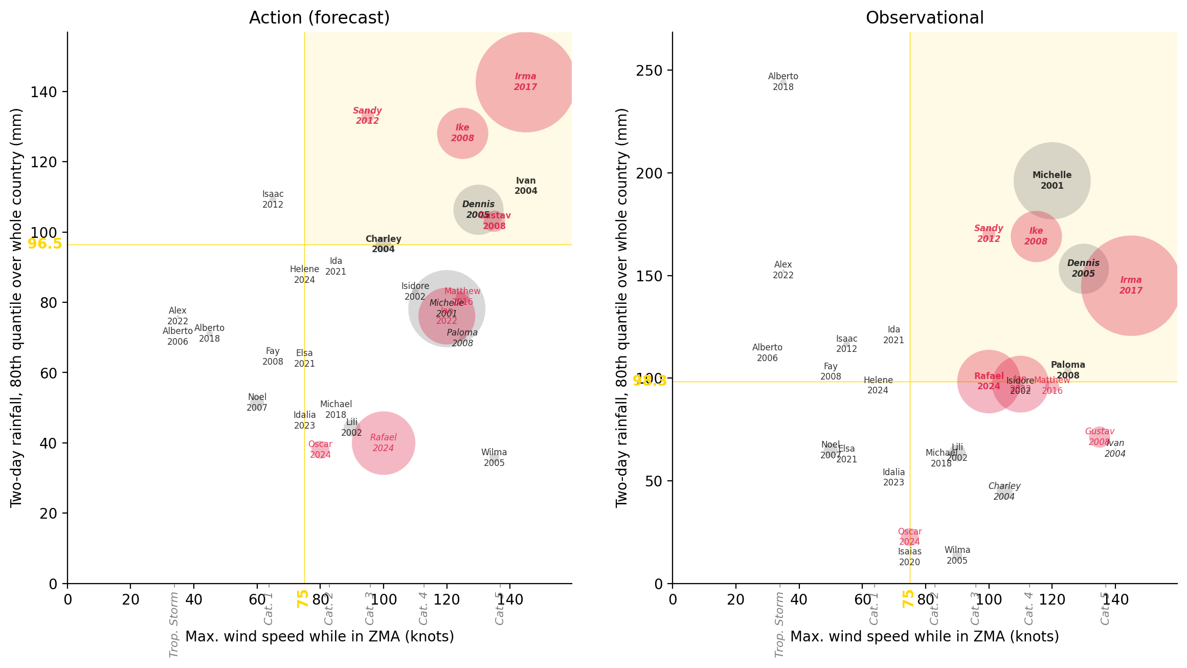
disp_selected_threshs(321972)| Action | Obsv. | CERF | Total Affected | |
|---|---|---|---|---|
| Storm | ||||
| Irma 2017 | Trig. | Trig. | Yes | 10,000,000 |
| Michelle 2001 | No trig. | Trig. | pre- | 5,900,012 |
| Rafael 2024 | No trig. | Trig. | Yes | 4,000,000 |
| Ian 2022 | No trig. | No trig. | Yes | 3,200,000 |
| Ike 2008 | Trig. | Trig. | Yes | 2,600,000 |
| Dennis 2005 | Trig. | Trig. | pre- | 2,500,000 |
| Gustav 2008 | Trig. | No trig. | Yes | 450,019 |
| Oscar 2024 | No trig. | No trig. | Yes | 320,000 |
| Lili 2002 | No trig. | No trig. | pre- | 281,470 |
| Charley 2004 | Trig. | No trig. | pre- | 244,005 |
| Noel 2007 | No trig. | No trig. | No | 192,488 |
| Matthew 2016 | No trig. | No trig. | Yes | 190,000 |
| Sandy 2012 | Trig. | Trig. | Yes | 162,605 |
| Wilma 2005 | No trig. | No trig. | pre- | 100,000 |
| Paloma 2008 | No trig. | Trig. | No | 49,445 |
| Isaac 2012 | No trig. | No trig. | No | 45,496 |
| Isidore 2002 | No trig. | No trig. | pre- | 42,500 |
| Alberto 2018 | No trig. | No trig. | No | 40,000 |
| Alex 2022 | No trig. | No trig. | No | 6,780 |
| Ivan 2004 | Trig. | No trig. | pre- | 3,245 |
| Michael 2018 | No trig. | No trig. | No | 540 |
| Isaias 2020 | No trig. | No trig. | No | 500 |
| Alberto 2006 | No trig. | No trig. | No | 268 |
| Ida 2021 | No trig. | No trig. | No | 0 |
| Elsa 2021 | No trig. | No trig. | No | 0 |
| Idalia 2023 | No trig. | No trig. | No | 0 |
| Helene 2024 | No trig. | No trig. | No | 0 |
| Dean 2007 | No trig. | No trig. | No | 0 |
| Fay 2008 | No trig. | No trig. | No | 0 |
As of July 2025 option 1b was chosen by the WG. Therefore, let’s look at this option again, this time with the readiness window built in.
blob_name = f"{PROJECT_PREFIX}/processed/nhc/monitors_nhc_chirpsgefs.parquet"
df_monitors_fcast = stratus.load_parquet_from_blob(blob_name)

df_stats_fcast_readiness = (
    df_monitors_fcast[df_monitors_fcast["lt_name"] == "readiness"]
    .groupby("atcf_id")
    .max()
    .reset_index()
    .dropna()
    .drop(columns=["issue_time", "lt_name"])
)
blob_name = f"{PROJECT_PREFIX}/processed/impact/emdat_cerf_upto2024.parquet"
df_impact = stratus.load_parquet_from_blob(blob_name)

df_storms = ibtracs.load_storms()
cols = ["sid", "atcf_id"]
df_storm_lookup = df_storms[cols].copy()

df_storm_lookup["atcf_id"] = df_storm_lookup["atcf_id"].str.lower()

df_stats_fcast_readiness_labelled = df_stats_fcast_readiness.merge(
    df_storm_lookup
)


df_stats_fcast_readiness_labelled["Readiness"] = (
    df_stats_fcast_readiness_labelled.apply(
        lambda row: (
            "Trig."
            if (
                # use actual readiness trigger (same as action)
                row["wind"]
                >= THRESHS["readiness"]["s"]
            )
            else "No trig."
        ),
        axis=1,
    )
)# Function to get trigger results with readiness analysis
def get_action_obsv_trig_results(index, impact_col="Total Affected"):
"""
Returns a dataframe with trigger results including readiness column
"""
df_disp = get_triggered_storms(index).copy()
df_disp["CERF"] = df_disp.apply(set_cerf_str, axis=1)
df_disp["Storm"] = (
df_disp["name"].str.capitalize() + " " + df_disp["year"].astype(str)
)
df_disp["Action"] = df_disp["fcast_trig"].apply(
lambda x: "Trig." if x else "No trig."
)
df_disp["Obsv."] = df_disp["obsv_trig"].apply(
lambda x: "Trig." if x else "No trig."
)
cols = ["sid","Storm", "Action", "Obsv.", "CERF", impact_col]
return df_disp[cols].sort_values(impact_col, ascending=False)
df_metrics
# Get results for option 1b (index 13136 from earlier analysis)
df_1b_with_readiness = get_action_obsv_trig_results(13136).merge(df_stats_fcast_readiness_labelled)# Optional: Create a styled display of the results
def display_styled_results(df_results, impact_col="Total Affected"):
"""
Display the results with styling if needed
"""
def color_df_extended(val):
if val == "Yes":
return "background-color: crimson"
elif val == "No":
return "background-color: dodgerblue"
elif val == "Trig.":
return "background-color: darkorange"
else:
return ""
cols_for_display = ["Readiness","Action", "Obsv.", "CERF", impact_col]
return (
df_results.set_index("Storm")[cols_for_display]
.style.bar(
subset=impact_col,
color="mediumpurple",
props="width: 150px;",
)
.map(color_df_extended)
.set_table_styles(
{
impact_col: [
{"selector": "th", "props": [("text-align", "left")]},
{"selector": "td", "props": [("text-align", "left")]},
]
}
)
.format({"Total Affected": "{:,}"})
)
# Display styled version if desired
display_styled_results(df_1b_with_readiness)| Readiness | Action | Obsv. | CERF | Total Affected | |
|---|---|---|---|---|---|
| Storm | |||||
| Irma 2017 | Trig. | Trig. | Trig. | Yes | 10,000,000 |
| Michelle 2001 | Trig. | Trig. | Trig. | pre- | 5,900,012 |
| Rafael 2024 | No trig. | No trig. | No trig. | Yes | 4,000,000 |
| Ian 2022 | Trig. | Trig. | Trig. | Yes | 3,200,000 |
| Ike 2008 | Trig. | Trig. | Trig. | Yes | 2,600,000 |
| Dennis 2005 | Trig. | Trig. | Trig. | pre- | 2,500,000 |
| Gustav 2008 | Trig. | Trig. | No trig. | Yes | 450,019 |
| Oscar 2024 | No trig. | No trig. | No trig. | Yes | 320,000 |
| Lili 2002 | No trig. | No trig. | No trig. | pre- | 281,470 |
| Charley 2004 | No trig. | No trig. | No trig. | pre- | 244,005 |
| Noel 2007 | No trig. | No trig. | No trig. | No | 192,488 |
| Matthew 2016 | Trig. | Trig. | Trig. | Yes | 190,000 |
| Sandy 2012 | No trig. | No trig. | No trig. | Yes | 162,605 |
| Wilma 2005 | Trig. | Trig. | No trig. | pre- | 100,000 |
| Paloma 2008 | Trig. | Trig. | Trig. | No | 49,445 |
| Isaac 2012 | No trig. | No trig. | No trig. | No | 45,496 |
| Isidore 2002 | No trig. | No trig. | No trig. | pre- | 42,500 |
| Alberto 2018 | No trig. | No trig. | No trig. | No | 40,000 |
| Alex 2022 | No trig. | No trig. | No trig. | No | 6,780 |
| Ivan 2004 | Trig. | Trig. | No trig. | pre- | 3,245 |
| Michael 2018 | No trig. | No trig. | No trig. | No | 540 |
| Alberto 2006 | No trig. | No trig. | No trig. | No | 268 |
| Ida 2021 | No trig. | No trig. | No trig. | No | 0 |
| Elsa 2021 | No trig. | No trig. | No trig. | No | 0 |
| Idalia 2023 | No trig. | No trig. | No trig. | No | 0 |
| Helene 2024 | No trig. | No trig. | No trig. | No | 0 |
| Fay 2008 | No trig. | No trig. | No trig. | No | 0 |
def calculate_joint_return_period(df_results):
    """
    Calculate the return period when any of the three triggers (Action, Obsv., Readiness) fires
    """
    # Create boolean columns for each trigger type
    df_calc = df_results.copy()
    df_calc["action_bool"] = df_calc["Action"] == "Trig."
    df_calc["obsv_bool"] = df_calc["Obsv."] == "Trig."
    df_calc["readiness_bool"] = df_calc["Readiness"] == "Trig."

    # Create combined trigger: TRUE if ANY of the three triggers fire
    df_calc["any_trig"] = (
        df_calc["action_bool"]
        | df_calc["obsv_bool"]
        | df_calc["readiness_bool"]
    )

    # Extract year from Storm column (assuming format "Name YYYY")
    df_calc["year"] = df_calc["Storm"].str.extract(r"(\d{4})").astype(int)

    # Get distinct years where any trigger fired
    triggered_years = df_calc[df_calc["any_trig"]]["year"].unique()
    n_triggered_years = len(triggered_years)

    # Calculate return period using Weibull formula
    # Total period: 2000-2024 = 25 years
    total_years = 25
    return_period = (total_years + 1) / n_triggered_years

    # print(f"Triggered years: {sorted(triggered_years)}")
    print(f"Number of triggered years: {n_triggered_years}")
    print(f"Total analysis period: {total_years} years (2000-2024)")
    print(f"Joint return period: {return_period:.2f} years")

    return {
        # "triggered_years": triggered_years,
        "n_triggered_years": n_triggered_years,
        "return_period": return_period,
        "df_with_any_trig": df_calc,
    }


# Calculate joint return period for Option 1b
joint_rp_results = calculate_joint_return_period(df_1b_with_readiness)
Number of triggered years: 7
Total analysis period: 25 years (2000-2024)
Joint return period: 3.71 years# Show detailed breakdown by trigger type
def analyze_trigger_breakdown(joint_results):
"""
Analyze which storms are triggered by which combination of triggers
"""
df_analysis = joint_results["df_with_any_trig"]
# Create trigger combination categories - use a more systematic approach
df_analysis["trigger_combo"] = "No trigger" # Default value
# First handle all triggered cases (any_trig == True)
triggered_mask = df_analysis["any_trig"]
# Use nested conditions to ensure mutually exclusive categories
df_analysis.loc[
triggered_mask
& df_analysis["action_bool"]
& df_analysis["obsv_bool"]
& df_analysis["readiness_bool"],
"trigger_combo",
] = "All three"
df_analysis.loc[
triggered_mask
& df_analysis["action_bool"]
& df_analysis["obsv_bool"]
& ~df_analysis["readiness_bool"],
"trigger_combo",
] = "Action + Obsv"
df_analysis.loc[
triggered_mask
& df_analysis["action_bool"]
& ~df_analysis["obsv_bool"]
& df_analysis["readiness_bool"],
"trigger_combo",
] = "Action + Readiness"
df_analysis.loc[
triggered_mask
& ~df_analysis["action_bool"]
& df_analysis["obsv_bool"]
& df_analysis["readiness_bool"],
"trigger_combo",
] = "Obsv + Readiness"
df_analysis.loc[
triggered_mask
& df_analysis["action_bool"]
& ~df_analysis["obsv_bool"]
& ~df_analysis["readiness_bool"],
"trigger_combo",
] = "Action only"
df_analysis.loc[
triggered_mask
& ~df_analysis["action_bool"]
& df_analysis["obsv_bool"]
& ~df_analysis["readiness_bool"],
"trigger_combo",
] = "Obsv only"
df_analysis.loc[
triggered_mask
& ~df_analysis["action_bool"]
& ~df_analysis["obsv_bool"]
& df_analysis["readiness_bool"],
"trigger_combo",
] = "Readiness only"
# Aggregate to year level to see which years had which trigger combinations
year_summary = (
df_analysis.groupby("year")
.agg(
{
"action_bool": "any", # True if ANY storm in that year triggered Action
"obsv_bool": "any", # True if ANY storm in that year triggered Obsv
"readiness_bool": "any", # True if ANY storm in that year triggered Readiness
"any_trig": "any", # True if ANY storm in that year triggered anything
"Total Affected": "sum", # Sum total affected for the year
}
)
.reset_index()
)
# Create year-level trigger combination categories
year_summary["year_trigger_combo"] = "No trigger"
triggered_years_mask = year_summary["any_trig"]
year_summary.loc[
triggered_years_mask
& year_summary["action_bool"]
& year_summary["obsv_bool"]
& year_summary["readiness_bool"],
"year_trigger_combo",
] = "All three"
year_summary.loc[
triggered_years_mask
& year_summary["action_bool"]
& year_summary["obsv_bool"]
& ~year_summary["readiness_bool"],
"year_trigger_combo",
] = "Action + Obsv"
year_summary.loc[
triggered_years_mask
& year_summary["action_bool"]
& ~year_summary["obsv_bool"]
& year_summary["readiness_bool"],
"year_trigger_combo",
] = "Action + Readiness"
year_summary.loc[
triggered_years_mask
& ~year_summary["action_bool"]
& year_summary["obsv_bool"]
& year_summary["readiness_bool"],
"year_trigger_combo",
] = "Obsv + Readiness"
year_summary.loc[
triggered_years_mask
& year_summary["action_bool"]
& ~year_summary["obsv_bool"]
& ~year_summary["readiness_bool"],
"year_trigger_combo",
] = "Action only"
year_summary.loc[
triggered_years_mask
& ~year_summary["action_bool"]
& year_summary["obsv_bool"]
& ~year_summary["readiness_bool"],
"year_trigger_combo",
] = "Obsv only"
year_summary.loc[
triggered_years_mask
& ~year_summary["action_bool"]
& ~year_summary["obsv_bool"]
& year_summary["readiness_bool"],
"year_trigger_combo",
] = "Readiness only"
# Show year-level breakdown
year_trigger_summary = (
year_summary.groupby("year_trigger_combo")
.agg({"year": lambda x: sorted(x.tolist()), "Total Affected": "sum"})
.round(0)
)
year_trigger_summary.columns = ["Years", "Total Affected"]
year_trigger_summary["Number of Years"] = year_trigger_summary[
"Years"
].apply(len)
print("\nYear-Level Trigger Combination Breakdown:")
print("=" * 50)
for combo, row in year_trigger_summary.iterrows():
print(
f"{combo}: {row['Number of Years']} years, {row['Total Affected']:,.0f} total affected"
)
if len(row["Years"]) > 0:
print(f" Years: {row['Years']}")
return year_trigger_summary
# Analyze the trigger breakdown
trigger_breakdown = analyze_trigger_breakdown(joint_rp_results)
trigger_breakdown
Year-Level Trigger Combination Breakdown:
==================================================
Action + Readiness: 1 years, 247,250 total affected
  Years: [2004]
All three: 6 years, 24,996,256 total affected
  Years: [2001, 2005, 2008, 2016, 2017, 2022]
No trigger: 8 years, 5,085,367 total affected
Years: [2002, 2006, 2007, 2012, 2018, 2021, 2023, 2024]| Years | Total Affected | Number of Years | |
|---|---|---|---|
| year_trigger_combo | |||
| Action + Readiness | [2004] | 247250 | 1 |
| All three | [2001, 2005, 2008, 2016, 2017, 2022] | 24996256 | 6 |
| No trigger | [2002, 2006, 2007, 2012, 2018, 2021, 2023, 2024] | 5085367 | 8 |